PCA: Preserve Variation in Fewer Dimensions
Expanded from PCA and LDA.pdf · View a handwritten page
In the K-means guide, we used measurements to compare points. With many measurements, comparing points can be hard to picture. Principal component analysis (PCA) combines those measurements into fewer new numbers, called coordinates, while keeping as much of the points' spread (variation) as possible. The new numbers combine original columns rather than simply selecting a few. We will first explain what PCA tries to maximize, then follow four points with two measurements each.
What PCA actually does
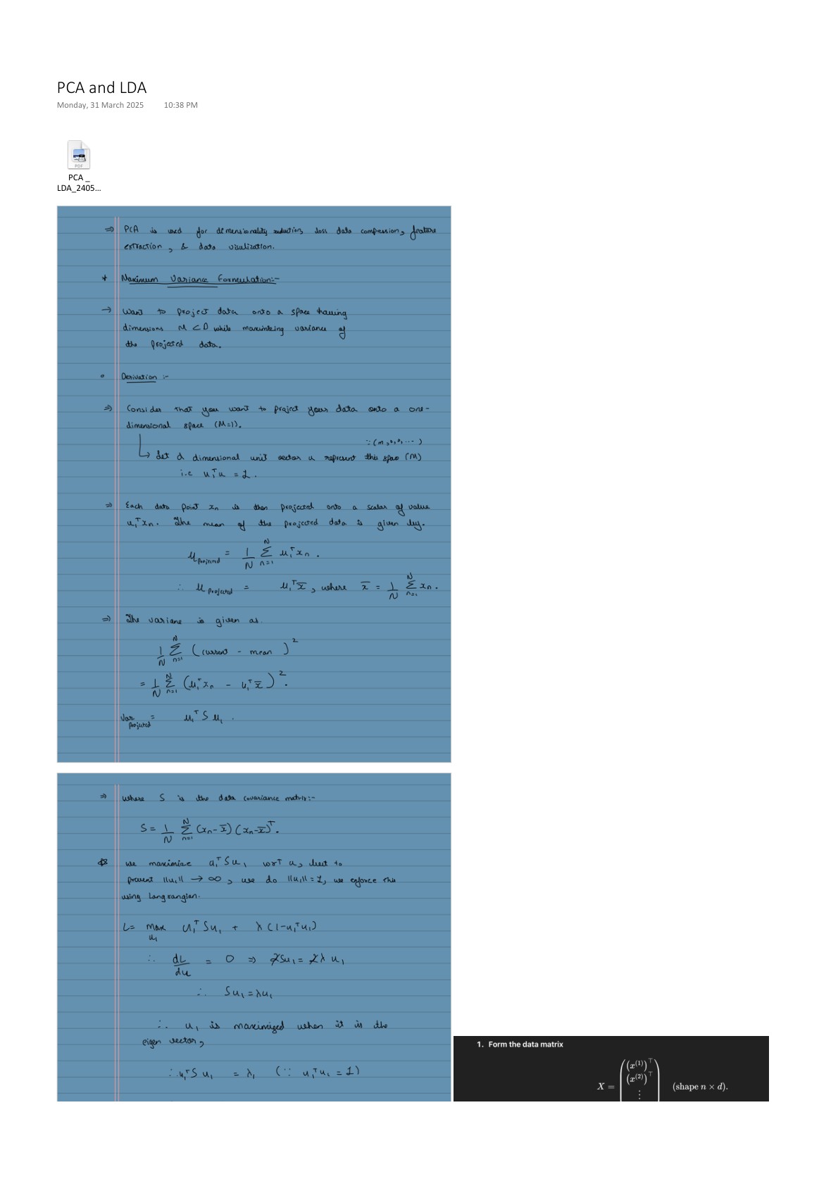
PCA creates new axes by combining measurements. For its first axis, it chooses a unit direction $v$ for a line through the data's mean, then projects each centered point onto that line. A point $x_i$ gets one score, $z_i=v^\top(x_i-\mu)$. PCA picks the direction that makes these scores spread out the most. This is the maximum-variance direction.
To see why the projected variance is $v^\top Sv$, let $X_c$ be the table of centered points and $S=X_c^\top X_c/(n-1)$ their sample covariance matrix. The score for all points together is $z=X_cv$. Since the points are centered, the scores also have mean zero. Their sample variance is:
So PCA's first component solves this problem:
The unit-length condition compares directions only; without it, we could make the scores larger just by lengthening $v$. To solve the constrained problem, introduce a Lagrange multiplier $\lambda$. Since $S$ is symmetric, the gradient of $v^\top Sv$ is $2Sv$:
Setting the gradient to zero gives $Sv=\lambda v$, so a maximizing direction must be an eigenvector of $S$. For a unit eigenvector $u$, the projected variance is $u^\top Su=\lambda$. Because $S$ is symmetric, its eigenvectors can be chosen perpendicular and unit length. Any unit direction is a combination $v=\sum_j a_j u_j$, with $\sum_j a_j^2=1$, so its variance is $v^\top Sv=\sum_j\lambda_j a_j^2$. This is a weighted average of the eigenvalues, so the maximum is the largest eigenvalue. The first principal component is its eigenvector.
Later components use the same goal, with the added condition that they be perpendicular to earlier components. We will calculate $S$ for four points and then find its first direction.
Start with two measurements per row
| Point | Measurement 1 | Measurement 2 | After subtracting means |
|---|---|---|---|
| A | 1 | 1 | (−1.5, −1.5) |
| B | 2 | 3 | (−0.5, 0.5) |
| C | 3 | 2 | (0.5, −0.5) |
| D | 4 | 4 | (1.5, 1.5) |
Each row is one point, and each column is one measurement. Both column means are 2.5. PCA subtracts each mean from its column, so the average value becomes zero. For point A, this gives $(1-2.5,1-2.5)=(-1.5,-1.5)$, as shown in the table. Centering shifts every point by the same amount, so the gaps between points stay the same. Keep the means so you can later convert PCA results back to the original measurements.
See how the measurements vary together
The variance of one measurement tells us how spread out its values are. Covariance tells us whether two measurements tend to move together. Here we use sample covariance, so divide by $n-1=3$. The squared centered values in the first column add to 5; the second column also adds to 5. To compare the columns, multiply their centered values row by row and add them: $2.25-0.25-0.25+2.25=4$. Dividing by 3 gives a covariance of $4/3$.
$X_c$ is the table of centered values. The diagonal entries ($5/3$) show the spread of each measurement. The off-diagonal entries ($4/3$) are positive, so the measurements tend to be above or below their averages together. If we divided by $n$ instead of $n-1$, all covariance values and eigenvalues would shrink by the same factor. The directions and explained-variance percentages would stay the same. This matrix now gives us what we need to find the direction where the data spread out most.
Find the direction for these four points
For this data, the derivation says to choose the eigenvector with the largest eigenvalue. The two eigenvectors and eigenvalues are:
The first direction follows the diagonal where both measurements increase together. The second follows the direction where they differ. Since $3$ is larger than $1/3$, the first direction contains more spread. Add the variance along both directions to get $3+1/3=10/3$. The first component keeps $3/(10/3)=\mathbf{90\%}$ of the sample variance. This is 90% of the dataset's total variation, not 90% of every point's details.
Reduce each point to one score, then rebuild it
We now keep only the first component. Since $v_1=(1,1)/\sqrt2$, each point's score is the sum of its two centered measurements divided by $\sqrt2$. For A, that is $(-1.5-1.5)/\sqrt2\approx-2.1213$.
| Point | First score | Reconstructed pair |
|---|---|---|
| A | −2.1213 | (1, 1) |
| B | 0 | (2.5, 2.5) |
| C | 0 | (2.5, 2.5) |
| D | 2.1213 | (4, 4) |
To reconstruct a point, start at the mean and move along the retained direction by its score: $\hat x=\mu+zv_1$. B and C both have score 0, so both return to the mean $(2.5,2.5)$. PCA can no longer tell them apart because their difference lies along the direction we dropped.
A and D lie on the retained line, so their reconstructions are exact. B and C each differ from their reconstruction by 0.5 in both measurements, giving squared error $0.5^2+0.5^2=0.5$ each and 1 in total. This equals $(n-1)\lambda_2=3\times(1/3)$: multiplying the discarded sample variance by $n-1=3$ gives the total squared error.

With several retained components, put their direction vectors into the columns of $V$. The scores $Z=X_cV$ are each point's new coordinates. Reconstructing with $ZV^\top+\mu$ maps those coordinates back to the original measurements. Flipping a direction's sign also flips its scores, so the reconstructed points stay the same.
The code below repeats the same steps: center the measurements, find the directions of greatest spread, keep the first direction, and reconstruct the points from their scores.
import numpy as np

X = np.array([[1., 1.], [2., 3.], [3., 2.], [4., 4.]])
mean = X.mean(axis=0)  # average of each measurement
centered = X - mean  # shift the averages to zero
values, vectors = np.linalg.eigh(centered.T @ centered / 3)
v = vectors[:, -1]  # eigh returns eigenvalues from smallest to largest
scores = centered @ v  # one score for each point
reconstructed = mean + np.outer(scores, v)  # approximate the original points
print(values[-1] / values.sum())  # fraction of variance kept: 0.9
print(np.sum((X - reconstructed)**2))  # total squared error: 1.0
Our example uses measurements with comparable units. With real data, centering and scaling are separate decisions. Centering subtracts the mean of each measurement. Scaling divides by a value such as its standard deviation, a measure of how spread out that measurement is. After scaling, differences are measured relative to each column's spread. This can help when columns use different units and you want equal relative differences to count similarly, but scaling also changes what PCA treats as important. Fit the means, scales, and PCA directions on training data, then reuse them for validation or new points so every point uses the same transformation.
You can also find the directions with singular value decomposition (SVD). It works directly on the centered data, without first building the covariance matrix.
What does PCA keep, and what can it lose?
PCA does not look at class labels. It keeps directions where the whole dataset varies most, even if that variation does not help separate the classes you care about. A direction with little overall variation can still distinguish classes, so keeping most of the variance does not guarantee a good classifier.
With $d$ measurements and $n$ points, centering leaves at most $n-1$ independent directions. So the number of nonzero components cannot exceed $\min(d,n-1)$. Choose how many to keep based on how much detail you need and what you will use the reduced data for.
If your goal is to separate known classes, use a method that takes the labels into account. The Fisher LDA guide explains how LDA chooses a projection to separate classes.
From the handwritten notes
This guide expands the relevant material in PCA and LDA.pdf. The complete original contains both topics; the blog treats PCA, LDA projection, and LDA classification separately.
View original page 1
Further reading: