Fisher LDA: Find a Projection That Separates Classes
Expanded from PCA and LDA.pdf · View a handwritten page
PCA keeps directions with a lot of overall spread. Fisher's linear discriminant analysis (LDA) asks a different question: on which line are the class averages far apart compared with the spread inside each class? It uses the labels to answer that question. We will build the matrices from ten points, derive the best direction, and check the result. A projection can help separate classes, but it does not guarantee that they stop overlapping.
Start with the labeled points in the notes
Each point belongs to class A or B. LDA uses those labels while it chooses a direction. Here are the ten points listed on page 4 of the original notes:
| Row | Class | $x_1$ | $x_2$ |
|---|---|---|---|
| A1 | A | 4 | 1 |
| A2 | A | 2 | 4 |
| A3 | A | 2 | 3 |
| A4 | A | 3 | 6 |
| A5 | A | 4 | 4 |
| B1 | B | 9 | 10 |
| B2 | B | 6 | 8 |
| B3 | B | 9 | 5 |
| B4 | B | 8 | 7 |
| B5 | B | 10 | 8 |
Average the measurements within each class. For A, the averages are $\mu_A=((4+2+2+3+4)/5,(1+4+3+6+4)/5)=(3,3.6)$. Doing the same for B gives $\mu_B=(8.4,7.6)$. The centers differ by $(5.4,4)$. A line along that gap would put the averages far apart, but it might also spread points from the same class far apart. LDA accounts for both.

Build the within-class scatter matrices
Each point $x_i$ is a column of measurements. A class's mean $\mu_c$ is the column of its average measurements. Subtract the mean of the point's own class to get its residual, $r_i=x_i-\mu_c$: the difference from the average in each measurement.
| Symbol | What it measures |
|---|---|
| $S_A$ | Spread of class A points around A's mean. |
| $S_B$ | Spread of class B points around B's mean. |
| $S_W=S_A+S_B$ | Total spread inside the two classes. W means “within.” |
| $S_{\mathrm{between}}$ | Spread of class means around the overall mean; defined in the multiclass section. |
Here B is the name of our second class, so $S_B$ measures spread inside class B, not the gap between classes. We write the between-class matrix as $S_{\mathrm{between}}$ to keep the meanings separate.
For any class $c$, add its residual outer products to form its scatter matrix:
This is a $d\times d$ matrix when each point has $d$ measurements. It records relationships between measurements, not between rows. Using each point's own class mean keeps the gap between classes out of this within-class measure.
In code, stack the residuals as rows of a matrix $R_c$. Then $S_c=R_c^\top R_c$: its entry $(j,k)$ adds the products $r_{ij}r_{ik}$ across the class. This is why the worked Python example uses Ac.T @ Ac and Bc.T @ Bc.
With two measurements, write a residual as the column vector $r_i=(r_{i1},r_{i2})^\top$. Multiply it by its row version to get that point's contribution to the scatter matrix:
The diagonal stores each squared difference. The off-diagonal stores the product of the two differences: it is positive when they have the same sign and negative when they have opposite signs. For A1, $\mu_A=(3,3.6)$ and $x_{A1}=(4,1)$, so $r_{A1}=(1,-2.6)$ and:
Repeat this for each class A point. The table lists the residual and the three distinct entries in its matrix contribution:
| Point | Residual $(r_1,r_2)$ | $r_1^2$ | $r_1r_2$ | $r_2^2$ |
|---|---|---|---|---|
| A1 | (1, −2.6) | 1 | −2.6 | 6.76 |
| A2 | (−1, 0.4) | 1 | −0.4 | 0.16 |
| A3 | (−1, −0.6) | 1 | 0.6 | 0.36 |
| A4 | (0, 2.4) | 0 | 0 | 5.76 |
| A5 | (1, 0.4) | 1 | 0.4 | 0.16 |
| Sum | 4 | −2 | 13.2 | |
Summing the three numeric columns gives $4$, $-2$, and $13.2$. Put those sums on the diagonal and in both off-diagonal positions to get class A's scatter matrix:
Now repeat the same steps using class B's mean, $\mu_B=(8.4,7.6)$:
| Point | Residual $(r_1,r_2)$ | $r_1^2$ | $r_1r_2$ | $r_2^2$ |
|---|---|---|---|---|
| B1 | (0.6, 2.4) | 0.36 | 1.44 | 5.76 |
| B2 | (−2.4, 0.4) | 5.76 | −0.96 | 0.16 |
| B3 | (0.6, −2.6) | 0.36 | −1.56 | 6.76 |
| B4 | (−0.4, −0.6) | 0.16 | 0.24 | 0.36 |
| B5 | (1.6, 0.4) | 2.56 | 0.64 | 0.16 |
| Sum | 9.2 | −0.2 | 13.2 | |
These columns sum to $9.2$, $-0.2$, and $13.2$, giving class B's scatter matrix:
$S_A$ measures spread inside A; $S_B$ measures spread inside B. Add them to get the total within-class scatter, $S_W$:
Each entry is an ordinary sum: $13.2=4+9.2$, $-2.2=-2-0.2$, and $26.4=13.2+13.2$. A negative off-diagonal entry is valid; it comes from opposite-sign residual products, not negative squared spread.
Scatter is a raw sum, not a covariance average. For example, A's sample covariance is $S_A/(5-1)$. We use the unnormalized $S_W$ in Fisher's criterion below. Dividing the whole matrix by one common positive number changes the criterion's value but not its best direction. Separately averaging classes with different sizes would change their relative weight.
Derive Fisher's separation score
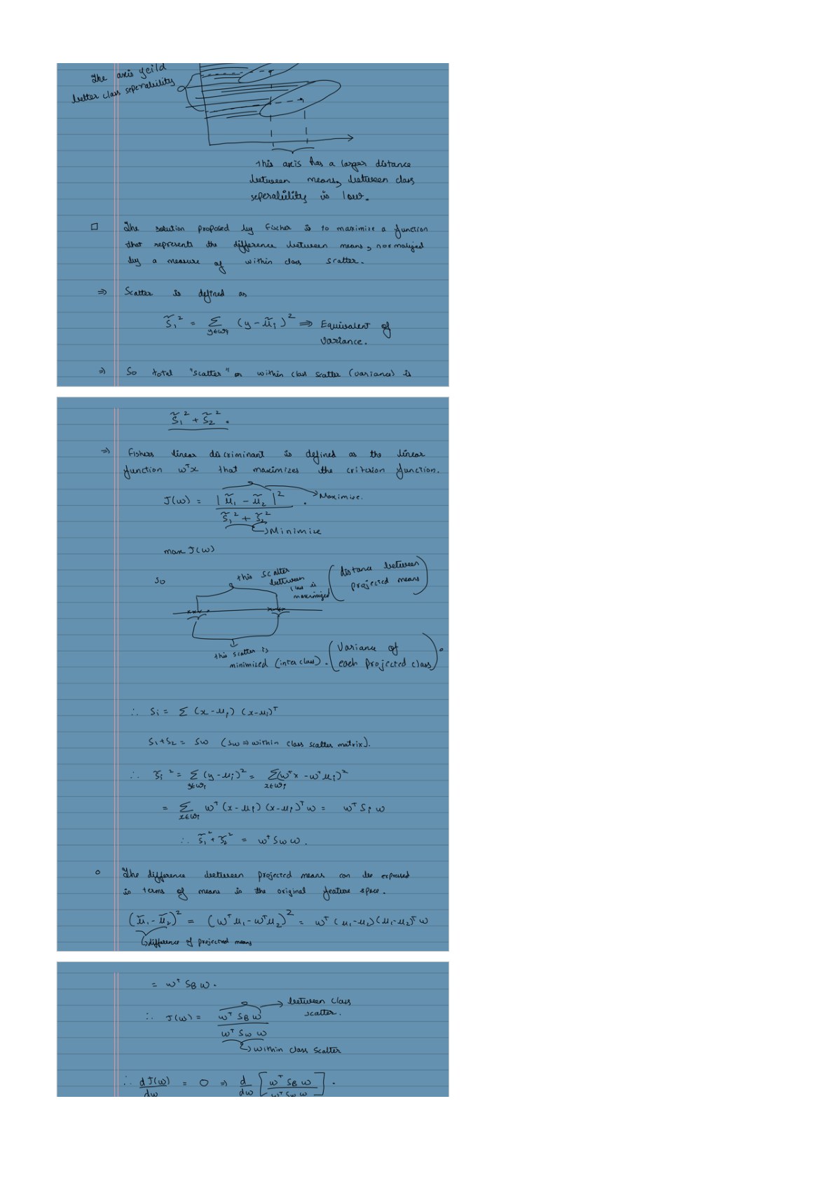
Let $w$ be a column of feature weights. A point gets one score, $z_i=w^\top x_i$. For two measurements, that means $z_i=w_1x_{i1}+w_2x_{i2}$. Averaging these scores within class $c$ gives:
Here $n_c$ is the number of points in class $c$. Define the mean-gap vector $g=\mu_B-\mu_A$. The gap between the two average scores is:
For point $i$, let $y_i$ be its class label. Its score's difference from its own class average is $z_i-\bar z_{y_i}=w^\top(x_i-\mu_{y_i})=w^\top r_i$. Square these differences and add them:
So Fisher's criterion is the squared gap between class averages divided by their total within-class spread, provided the denominator is positive:
A large numerator means the projected class averages are far apart; a small denominator means points stay close to their own class averages. Multiplying $w$ by a nonzero scalar leaves the ratio unchanged. This score is not a probability or a prediction accuracy.
Why scatter is symmetric, but not always positive definite
These are different properties. Symmetry is guaranteed by the way we build $S_W$. Positive definiteness needs an additional condition on the data.
Each residual $r_i$ is a column vector. Its outer product $r_ir_i^\top$ has the same entry in positions $(j,k)$ and $(k,j)$, because $r_{ij}r_{ik}=r_{ik}r_{ij}$. Transposing it therefore changes nothing. Adding these symmetric matrices keeps them symmetric:
To understand positivity, look at what a direction $w$ measures. The number $w^\top r_i$ is a point's difference from its own class mean after projection. The denominator adds the squares of those differences:
A sum of squares cannot be negative, so $S_W$ is always positive semidefinite. “Semidefinite” allows a nonzero $w$ to give zero. Positive definite means the sum is strictly positive for every nonzero $w$.
Positive definiteness is the stronger case: every positive-definite matrix is also positive semidefinite, but the reverse is not true. These terms describe $w^\top S_Ww$, not whether every matrix entry is positive. Our actual scatter has negative off-diagonal entries and is still positive definite.
The sum is zero only when every projected residual is zero. For $S_W$ to be positive definite, the residuals must therefore have variation in every feature direction. Equivalently, the residual matrix $R$ whose rows are $r_i^\top$ must have full column rank: $Rw=0$ must imply $w=0$.
Why our two-measurement example meets that condition
We can check it using just two of the residuals from the class A table: $r_{A1}=(1,-2.6)^\top$ and $r_{A2}=(-1,0.4)^\top$. For a direction $w=(w_1,w_2)^\top$, their projected residuals are:
For both to be zero, the first equation requires $w_1=2.6w_2$ and the second requires $w_1=0.4w_2$. Hence $2.2w_2=0$, which forces $w_2=0$ and then $w_1=0$. No nonzero direction can make both squares vanish. At least one is positive, and the other points add only nonnegative squares. That proves our $S_W$ is positive definite.
Derive the best direction with gradients
The inverse-based derivation assumes $S_W$ is positive definite, as we just proved for our example. Also assume the class means differ, so $g\ne0$. These conditions let us divide by positive within-class spread and invert $S_W$.
Because rescaling $w$ does not change $J(w)$, choose a convenient scale: $w^\top S_Ww=1$. The problem becomes:
The mean gap is $w^\top g=\sum_j w_jg_j$, whose gradient with respect to the weights is $g$. Squaring it gives gradient $2g(g^\top w)$ by the chain rule.
Where the denominator's gradient comes from
The class means, residuals, and $S_W$ are fixed training-data quantities here. We differentiate only with respect to $w$. Call the denominator $D(w)=w^\top S_Ww$ and use its sum-of-squares form.
For one residual, $w^\top r_i=\sum_j w_jr_{ij}$. Differentiating with respect to each weight gives the column of coefficients $r_i$. The chain rule for its square supplies the factor of 2:
Add the gradient contributions from all points. The scalar $w^\top r_i$ equals $r_i^\top w$, so we can write $r_i(w^\top r_i)=r_ir_i^\top w$:
This also explains the usual matrix shortcut. For any fixed matrix $M$, the weights appear twice in $w^\top Mw$. The product rule gives one contribution from the left copy, $Mw$, and one from the right copy, $M^\top w$:
With $M=S_W$ and $S_W^\top=S_W$, those contributions are identical and add to $2S_Ww$. Symmetry is enough for this gradient identity; positive definiteness is needed for the inverse-based optimization, not for differentiation. Here is the same result using our matrix entries:
The gradient is the column of partial derivatives with respect to the weights. To include the constraint, introduce a Lagrange multiplier $\lambda$ and set both derivatives of the Lagrangian to zero:
Divide the gradient equation by 2:
Which quantity is the eigenvector?
$w$ is the eigenvector; $\lambda$ is the eigenvalue. An eigenvector is a nonzero vector whose product with a matrix is a scalar multiple of that same vector: $Mw=\lambda w$. The vector specifies a direction, while the eigenvalue gives the multiplier. They are not interchangeable.
| Quantity | Type and meaning |
|---|---|
| $w$ | A $d\times1$ vector of projection weights. Its direction tells us how to combine the measurements into one score. |
| $\lambda$ | A scalar eigenvalue: one number. For an eigenvector in this problem, it equals the Fisher separation score. |
| $gg^\top$ | A $d\times d$ mean-gap matrix, with $g=\mu_B-\mu_A$. It represents the binary numerator $(w^\top g)^2$. |
| $S_W$ | A $d\times d$ matrix of within-class scatter. |
| $w^\top S_Ww$ | A scalar measuring within-class spread after projection. It is not the matrix whose eigenvector we choose. |
The equation $gg^\top w=\lambda S_Ww$ is a generalized eigenvector equation involving two matrices. With invertible $S_W$, multiply it by $S_W^{-1}$ to see the ordinary eigenvector form:
Thus $w$ is an eigenvector of the within-class-adjusted mean-gap matrix $M$, not necessarily an eigenvector of $S_W$ itself. In numerical code, solve the generalized problem directly rather than explicitly forming the inverse.
Why the eigenvalue equals the Fisher score
For a vector satisfying the generalized equation, multiply both sides by $w^\top$:
Under the chosen constraint $w^\top S_Ww=1$, this reduces to $\lambda=(w^\top g)^2$. Without that normalization, the ratio above is the score. Rescaling an eigenvector changes its length but leaves its direction and this ratio unchanged.
What does the largest-eigenvalue direction optimize?
Choose the eigenvector with the largest generalized eigenvalue, because that eigenvalue is its Fisher score. The goal is a large projected gap between class means relative to the spread inside the classes. It is not two independent goals of making between-class spread as large as possible and within-class spread as small as possible.
A direction with a big mean gap can also spread each class widely; one with tiny within-class spread can put both means together. The ratio balances these effects. Normalizing within-class spread to 1 lets us compare the mean gaps on a common spread scale. This differs from PCA, which maximizes the overall data variance without class labels.
For our data, the maximizing unit direction is $v\approx(0.919559,0.392951)^\top$, while the largest eigenvalue is $\lambda_{\max}\approx3.131370$. The two entries of $v$ are the feature weights; the single number $\lambda_{\max}$ measures their separation-to-scatter ratio. The worked calculation below obtains these values.
A direction with $g^\top w=0$ has score 0. Since the class means differ, the maximum is positive. For that maximizing eigenvector, $\lambda>0$, and the generalized equation gives:
Solve and check the direction for our points
For our points, the total within-class scatter is $S_W=\begin{bmatrix}13.2&-2.2\\-2.2&26.4\end{bmatrix}$ and the mean gap is $g=(5.4,4)^\top$. Find $u=S_W^{-1}g$ by solving a linear system instead of forming an inverse:
That matrix equation is just these two scalar equations:
The solution is $u\approx(0.440461,0.188220)^\top$. It points in the right direction, but it is not scaled to the constraint used in the gradient derivation. That scale would be $w=u/\sqrt{g^\top u}$, giving $w^\top S_Ww=1$. For plotting, use ordinary unit length instead:
These normalizations give the same direction and Fisher score. A point's plotted score is $z=v^\top x=0.919559x_1+0.392951x_2$. For A1, that is approximately $0.919559(4)+0.392951(1)=4.0712$.
On this line, class A's average score is about 4.1733 and class B's is about 10.7107. The direction separates the averages while accounting for how widely points spread within each class.
Trace the initial coordinates, delta, and projected coordinates
The initial coordinates here are the class means, $\mu_A=(3,3.6)^\top$ and $\mu_B=(8.4,7.6)^\top$. Their original two-coordinate difference is:
Each table row uses a different candidate weight vector $w=(w_1,w_2)^\top$. It is a separate projection, not a step in an iterative coordinate update. The bars on $\bar z_A$ and $\bar z_B$ mark class-average scores. Their formulas are $\bar z_A=w^\top\mu_A$ and $\bar z_B=w^\top\mu_B$; substitute the two entries of each class mean to get:
$\Delta$ is the gap between the new class-mean coordinates, not a displacement added to the original point. The denominator uses the same within-class matrix for every row:
| Candidate direction | Original → new class-mean coordinates | How the projected gap $\Delta$ is obtained | Fisher score calculation |
|---|---|---|---|
| First measurement only $w=(1,0)$ | A starts at $(3,3.6)$. $\begin{aligned}\bar z_A&=1(3)\\&\quad+0(3.6)\\&=3.\end{aligned}$ B starts at $(8.4,7.6)$. $\begin{aligned}\bar z_B&=1(8.4)\\&\quad+0(7.6)\\&=8.4.\end{aligned}$ | $\Delta=8.4-3$ $=5.4$. | $D=13.2$ $J=29.16/13.2$ $=2.2091$. |
| Second measurement only $w=(0,1)$ | A starts at $(3,3.6)$. $\begin{aligned}\bar z_A&=0(3)\\&\quad+1(3.6)\\&=3.6.\end{aligned}$ B starts at $(8.4,7.6)$. $\begin{aligned}\bar z_B&=0(8.4)\\&\quad+1(7.6)\\&=7.6.\end{aligned}$ | $\Delta=7.6-3.6$ $=4$. | $D=26.4$ $J=16/26.4$ $=0.6061$. |
| Mean-gap direction $w=(5.4,4)$ | A starts at $(3,3.6)$. $\begin{aligned}\bar z_A&=5.4(3)\\&\quad+4(3.6)\\&=30.6.\end{aligned}$ B starts at $(8.4,7.6)$. $\begin{aligned}\bar z_B&=5.4(8.4)\\&\quad+4(7.6)\\&=75.76.\end{aligned}$ | $\Delta=75.76-30.6$ $=45.16$. | $D=712.272$ $J=2039.4256/712.272$ $\approx2.8633$. |
| Fisher direction $w=v$ above | A starts at $(3,3.6)$. $\begin{aligned}\bar z_A&\approx0.919559(3)\\&\quad+0.392951(3.6)\\&\approx4.1733.\end{aligned}$ B starts at $(8.4,7.6)$. $\begin{aligned}\bar z_B&\approx0.919559(8.4)\\&\quad+0.392951(7.6)\\&\approx10.7107.\end{aligned}$ | $\Delta\approx10.7107-4.1733$ $\approx6.5374$. | $D\approx13.6483$ $\Delta^2\approx42.7379$ $J\approx42.7379/13.6483$ $\approx3.1314$. |
For example, the mean-gap row computes $\bar z_A=5.4(3)+4(3.6)=30.6$ and $\bar z_B=5.4(8.4)+4(7.6)=75.76$. Its large projected gap alone does not make it the best choice: these weights are not unit-normalized, and their within-class scatter also grows. Rescaling the weights changes $\Delta^2$ and $D$ by the same factor, leaving $J$ unchanged.
The Fisher direction gives $J(v)=g^\top u\approx3.131370$. Pointing directly from one class mean to the other gives a smaller score because it does not adjust for within-class spread.
Plotting all ten scores makes that separation easier to see:

import numpy as np

A = np.array([[4,1], [2,4], [2,3], [3,6], [4,4]], dtype=float)
B = np.array([[9,10], [6,8], [9,5], [8,7], [10,8]], dtype=float)
ma, mb = A.mean(0), B.mean(0)
Ac, Bc = A-ma, B-mb
scatter_a = Ac.T @ Ac
scatter_b = Bc.T @ Bc
within = scatter_a + scatter_b
gap = mb - ma
u = np.linalg.solve(within, gap)  # Solve within @ u = gap; no inverse is formed.
v = u / np.linalg.norm(u)
print(scatter_a)  # [[4, -2], [-2, 13.2]]
print(scatter_b)  # [[9.2, -0.2], [-0.2, 13.2]]
print(within)  # [[13.2, -2.2], [-2.2, 26.4]]
print(v)       # [0.91955932, 0.39295122]
print(gap @ u) # maximum Fisher score: 3.1313700384
Generalize the same idea to several classes
With $C$ classes, keep two separate measures: spread inside each class and spread of the class averages. Let class $c$ have $n_c$ points and mean $\mu_c$, with $n=\sum_c n_c$ total points. The overall mean is:
Add all class scatter matrices for $S_W$. For $S_{\mathrm{between}}$, compare each class mean with the overall mean and weight it by the class's size:
For two classes, this definition simplifies to $S_{\mathrm{between}}=(n_An_B/n)gg^\top$. In our example it is $2.5gg^\top$, or $\begin{bmatrix}72.9&54\\54&40\end{bmatrix}$. This is different from class B's scatter $S_B$. The factor 2.5 scales the binary Fisher criterion but does not change its best direction.
For multiple classes, maximize the ratio $R(w)=w^\top S_{\mathrm{between}}w/(w^\top S_Ww)$. With positive-definite $S_W$, normalize the denominator to 1 and differentiate:
Choose directions with the largest generalized eigenvalues. For several components, they can be chosen to satisfy $w_i^\top S_Ww_j=0$ for $i\ne j$. That means they are perpendicular under the within-class spread measure, but need not make a right angle in the ordinary geometric sense. PCA's axes are perpendicular in the input coordinates used for fitting.
The same equation can be written $(S_W^{-1}S_{\mathrm{between}})w=\lambda w$. This is useful algebraically, but $S_W^{-1}S_{\mathrm{between}}$ is not generally symmetric. In numerical code, solve the symmetric generalized eigenproblem directly rather than forming that inverse product and passing it to an ordinary symmetric eigensolver.
Why at most $C-1$ directions? The class-mean offsets obey $\sum_c n_c(\mu_c-\mu)=0$, so they cannot all be independent. Their span has at most $C-1$ dimensions. With $d$ input measurements, the number of positive between-class directions is therefore at most $\min(d,C-1)$, and it can be smaller. Two classes give at most one.
From the handwritten notes
This guide expands the relevant material in PCA and LDA.pdf. The complete original contains both topics; the blog treats PCA, LDA projection, and LDA classification separately.
View original page 3
Further reading: