Bagging & Random Forests
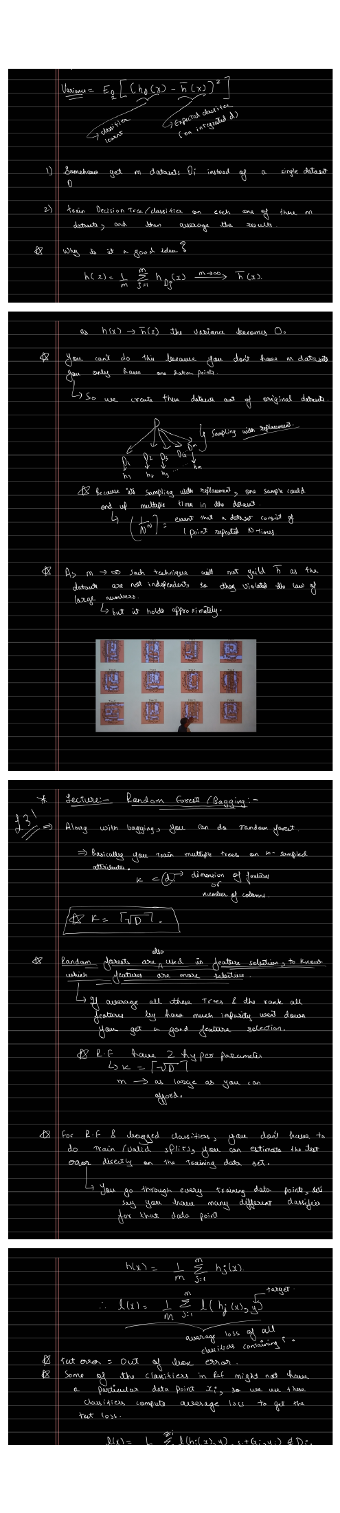
The scan motivates ensembles through variance. Keep two averages separate: averaging predictions from many trees, and averaging over hypothetical training datasets to define statistical variance.
Variance describes changing predictions across training sets
Hold one input fixed, retrain a model on different samples, and record its predictions. Their spread around their own average is the model’s variance at that input. The average itself can still be systematically wrong, so reducing spread does not guarantee accuracy.
Resample the available rows
A bootstrap draws rows with replacement: a sample of four rows might contain IDs [2, 2, 4, 1]. Fit a model to each resample and combine its predictions with the others.
Resamples can be drawn independently conditional on the observed dataset. As their number grows, their average approaches an expectation based on that dataset. The dataset itself is still random, so this limit can retain variance and bias. The law of large numbers has not been violated.
Average several perturbed predictions
A synthetic illustration: thin curves are generated by adding perturbations to a reference signal. The bold curve is their actual running average. No trees are trained here.
The readout is mean squared deviation from the synthetic reference, not an estimate of statistical variance over repeated training datasets. It need not fall with every added curve. The ensemble variance formula makes the role of correlation explicit.
Randomize candidate features at each split
A random forest restricts each node’s split search to a random subset of features. This can reduce shared mistakes, but hiding useful features can weaken synthetic curves. The subset size is a tuning choice; a square-root rule is a common classification heuristic, not the definition of a forest.
Combine held-out predictions before measuring error
For each training row, select only trees whose bootstrap samples omitted it. Combine their predictions first, then compare with that row’s target. Finally average the row losses.
For example, OOB regression predictions 2 and 4 average to 3. If the target is 3, their ensemble squared error is zero. Averaging the two individual squared errors would instead give 1, which evaluates a different predictor.
OOB performance is a useful internal estimate, not a guaranteed unbiased final test. Preprocessing, groups, time order, and repeated tuning still require an appropriate evaluation design.
Read feature scores and uncertainty with care
Impurity importance can favor features with many possible splits. Use explainability tools according to the question, and consider held-out permutation importance for predictive reliance. Variation between tree predictions is also not automatically a calibrated prediction interval.
For a fitted example with row-specific predictions and errors, see the out-of-bag calculation.
Sources and next steps
- Cornell: Bagging — Lecture companion for resampling and aggregation.
- Breiman: Random Forests — Correlation and out-of-bag evaluation.
- Permutation importance — Why impurity importance and held-out predictive reliance differ.