Boosting & AdaBoost

September 2026 · 4 min read

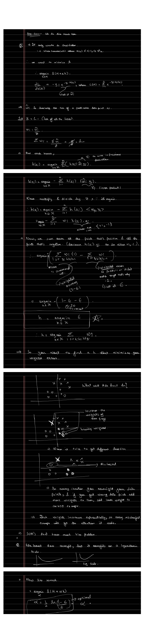
The scan connects two ideas: adding a small model to an existing prediction, and choosing that addition to reduce a loss. Use this page to read the notation; the linked chapters contain the worked derivations.

Keep the old model and add a correction

Call the current prediction function $F$, the next small learner $h$, and its step size $\alpha$. An additive update is:

For example, a prediction of 5 plus a correction of 2 with step size 0.1 becomes 5.2. The new learner supplies a correction, not a replacement prediction.

Ask which correction reduces the chosen loss

For half squared error, the negative derivative with respect to a row’s current prediction is its residual: target minus prediction. If the target is 7 and the prediction is 5, that correction target is +2.

A shallow tree cannot generally match every row’s ideal correction independently. Gradient boosting fits an approximation within its tree family. The functional gradient descent derivation and Gradient Boosting notes explain why the residual appears and how classification differs.

The regression loop

start with the mean training target
repeat:
    compute target minus current prediction for each row
    fit a small regression tree to those residuals
    add a learning-rate-scaled tree prediction
stop according to validation performance

This loop is for squared-error regression. Other losses require their own correction targets and possibly different leaf updates.

AdaBoost changes example weights

Binary AdaBoost uses labels and stump predictions of −1 or +1. It fits a learner under the current example weights, gives it a vote based on its weighted error, then increases the relative weight of missed examples.

In the figure, $\varepsilon$ is that weighted error and $\alpha$ is the new learner’s vote strength. Their formula and a five-row calculation are introduced in the worked AdaBoost rounds.

Read the algorithm’s boundary cases

Initialize weights uniformly and normalize them after each update. A perfect learner needs explicit handling instead of an infinite vote. A learner with error 0.5 earns no vote; one above 0.5 must be rejected, refitted, or have its binary predictions flipped.

The diagram stops when it reaches zero training error. This is a teaching choice: exponential loss can continue decreasing after every label is classified correctly.

Keep the training guarantee separate from generalization

If every round beats 50% weighted error by at least the same positive amount, the standard AdaBoost training-error bound decreases exponentially with rounds. The bound and its assumptions are written out in the ensemble chapter.

This does not imply a guaranteed test-error curve or slow overfitting. Repeatedly misclassified noisy labels can attract large weights. Validate the number of rounds and the capacity of the weak learner.

Continue with gradient-boosted machines for loss-specific leaf values and training controls.

Sources and next steps

• Cornell: Boosting — Lecture connection between additive models and loss minimization.
• Schapire: The Boosting Approach — AdaBoost updates, margins, and training-error guarantees.