CART, Complexity & Pruning
The scan connects three ideas: a leaf’s prediction, an efficient search over thresholds, and the cost of keeping extra leaves. This companion works through each one with small, explicit datasets. The numeric examples are teaching additions; the original scan remains below.
Why a regression leaf predicts an average
For targets 2, 4, and 9, the mean is 5. Predicting 5 gives squared errors 9, 1, and 16, totaling 26. Why choose 5? For any constant prediction c, the error decomposes into a fixed part plus a nonnegative penalty:
The minimum is therefore at c = 5. More generally, for rows S with target mean $\bar y_S$, the minimized total squared error is
This statement assumes equal observation weights and squared-error loss. A different loss or weighting rule can change the optimal leaf prediction. If the split score uses mean squared error, weight each child by its row fraction. If it uses total squared error, add the child totals directly.
Compare two actual regression splits
Assign the three targets to ordered feature values: (x, y) = (1, 2), (2, 4), (3, 9). Test the rule x < t. Any threshold between consecutive feature values makes the same partition of these training rows; use midpoints 1.5 and 2.5.
No split
Targets: [2, 4, 9]
Predict 5 for every row.
SSE = 9 + 1 + 16 = 26
x < 1.5
Left [2] → predict 2
Right [4, 9] → predict 6.5
SSE = 0 + 6.25 + 6.25 = 12.5
x < 2.5
Left [2, 4] → predict 3
Right [9] → predict 9
SSE = 1 + 1 + 0 = 2
Avoid rescanning every candidate’s rows
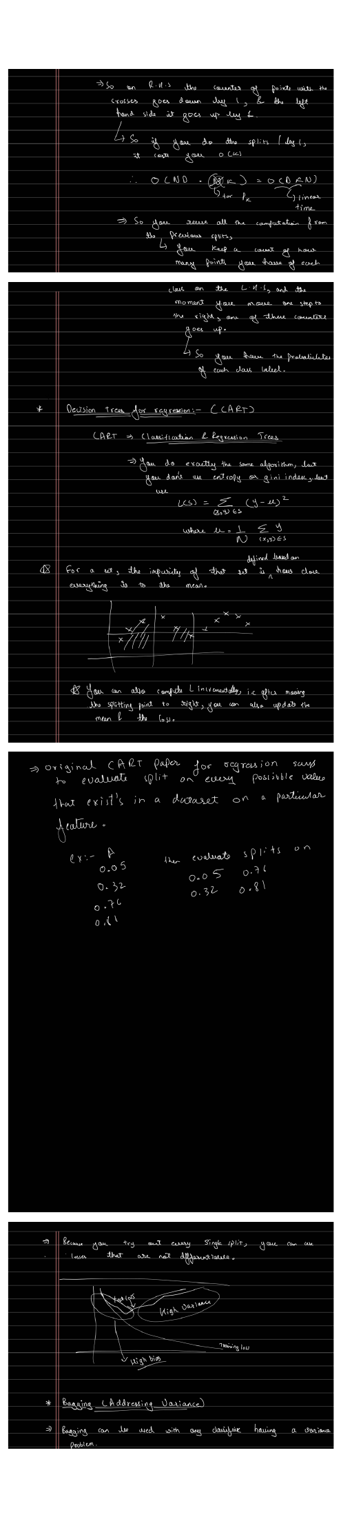
Now switch to classification to make the running counts visible. Let N be this node’s row count, D its feature count, and K the number of classes. For each feature, at most N − 1 boundaries can separate nonempty children. Recounting N labels at every boundary costs O(N²); scanning K class proportions for each score adds O(NK). A naive search over D features therefore costs O(D(N² + NK)), apart from smaller sorting work in the usual comparison-sort setting.
Sort a feature once in O(N log N). Start with every row on the right. Moving one row of class A increments left[A] and decrements right[A]; no other class counter changes. Those two counter updates take constant time. Scoring each candidate from all K counts costs O(K), giving O(D(N log N + NK)) for the node’s full search. This is a per-node calculation, not the cost of growing an entire tree.
Trace the nine legal boundaries
Use x = 1, 2, …, 10 and labels [A, A, B, A, B, B, A, B, B, B]. The parent has four A and six B rows, so its Gini impurity is 1 − 0.4² − 0.6² = 0.48. These values supply a reproducible companion example; they are not transcribed training data from the scan.
After moving k rows left, test t = k + 0.5 for k = 1 through 9. A child with class proportions pₐ and pᵦ has Gini 1 − pₐ² − pᵦ². Combine the child impurities with their row fractions:
At k = 2, the left counts are (2, 0), so GL = 0. The right counts are (2, 6), so GR = 1 − (2/8)² − (6/8)² = 0.375. The weighted score is (2/10) × 0 + (8/10) × 0.375 = 0.3, giving a reduction of 0.18. Exhausting the nine candidates confirms that t = 2.5 is best.
Rows are sorted by x. Read the cards left to right, then continue on the next line. “L” and “R” identify the current child.
Worked candidate: x < 2.5. The second A row has moved: left[A] +1, right[A] −1.
Left · 2 rows
Gini: 0.000000
Right · 8 rows
Gini: 0.375000
Count bars share the scale 0–6 rows. Green is class A; orange is class B. Bar length shows a count, not a class probability.
Reduction: 0.480000 − 0.300000 = 0.180000
Best after all nine candidates: x < 2.5, weighted Gini 0.300000.
Compare every legal candidate
| Threshold t | Left A / B | Right A / B | Weighted Gini | Reduction |
|---|---|---|---|---|
| 1.5 | 1 / 0 | 3 / 6 | 0.400000 | 0.080000 |
| 2.5 | 2 / 0 | 2 / 6 | 0.300000 | 0.180000 |
| 3.5 | 2 / 1 | 2 / 5 | 0.419048 | 0.060952 |
| 4.5 | 3 / 1 | 1 / 5 | 0.316667 | 0.163333 |
| 5.5 | 3 / 2 | 1 / 4 | 0.400000 | 0.080000 |
| 6.5 | 3 / 3 | 1 / 3 | 0.450000 | 0.030000 |
| 7.5 | 4 / 3 | 0 / 3 | 0.342857 | 0.137143 |
| 8.5 | 4 / 4 | 0 / 2 | 0.400000 | 0.080000 |
| 9.5 | 4 / 5 | 0 / 1 | 0.444444 | 0.035556 |
For equal feature values, move the entire tied group before testing its boundary. Otherwise a proposed cut would pretend to separate identical values. The numeric midpoint must also be representable and reproduce the intended comparison; the threshold-search implementation note covers those edge cases and missing-value policy.
When K is fixed, sorting dominates the count-based node search. With many classes, Gini can avoid a full K-count scan by maintaining the sum of squared counts. Incrementing count c changes c² by 2c + 1; decrementing it changes c² by −2c + 1. This is an additional optimization, distinct from merely updating the counts.
For regression, the analogous running quantities are count n, target sum S, and squared-target sum Q. A nonempty child’s SSE is Q − S²/n. Moving one target updates all three quantities on each side. For targets [2, 4], n = 2, S = 6, Q = 20 gives SSE = 20 − 36/2 = 2. Direct subtraction can lose precision for very large, nearly equal targets; use suitable centering or stable numerical updates in a production implementation.
Give extra leaves a reason to stay
Return to the three-row regression example. Suppose the current tree is the two-leaf tree at t = 2.5. Compare keeping it with replacing its root by one leaf. Use the explicitly unnormalized cost R(T) + α times the number of leaves, where R is total training SSE and α ≥ 0:
Keeping the split is cheaper when α < 24. At α = 24 the costs tie; above 24, pruning is cheaper. For example, α = 10 gives 22 versus 36, while α = 30 gives 62 versus 56. This compares these two trees only; it does not claim to enumerate every possible larger tree.
Normalization changes the numerical cutoff. Dividing the training error by all three rows gives 2/3 + 2α versus 26/3 + α, with a tie at α = 8. Do not transfer “24” into a library’s pruning parameter without checking its impurity and sample-weight convention. scikit-learn’s pruning documentation defines its weighted leaf-impurity objective.
Depth limits and minimum leaf sizes restrict growth before a split is made. Post-pruning removes branches from an already grown tree. Choose these controls using validation data; a better penalized training score alone does not prove better generalization. The full pruning chapter develops the sequence of candidate subtrees.
Read the scan’s depth sketch as a tendency
A shallow tree may miss a useful boundary. A deep tree can represent finer patterns but may change substantially when its training sample changes. The scan’s training/test-error sketch illustrates that tradeoff; it is not an empirical curve for either toy dataset here. A deep tree need not overfit every dataset, and pruning cannot identify “noise” without an evaluation criterion.
Reproduce all classification split scores in Python
labels = list("AABABBABBB")
left = {"A": 0, "B": 0}
right = {"A": labels.count("A"), "B": labels.count("B")}
def gini(counts):
    n = sum(counts.values())
    return 1 - sum((c/n)**2 for c in counts.values())

for k, label in enumerate(labels[:-1], start=1):
    left[label] += 1
    right[label] -= 1
    weighted = (k*gini(left) + (10-k)*gini(right)) / 10
    print(k + 0.5, left, right, round(weighted, 6),
          round(0.48 - weighted, 6))
# Minimum weighted Gini: 0.3 at threshold 2.5.
Each child is nonempty in this loop, so the impurity function never divides by zero. At initialization, display an empty-child state instead of treating it as a candidate.
Next, bagging combines predictions from separately fitted trees.
Sources and next steps
- Cornell’s tree lecture — Regression leaves and the motivation for controlling tree size.
- scikit-learn tree documentation — Pruning and implementation context.