3. The Mathematics: Where the Formulas Come From

September 2026 · Note 3 / 5 · 11 min read

Notes on StatQuest with Josh Starmer · The Mathematics: Where the Formulas Come From · 27:24 video. Original explanations and redrawn figures accompany the video.

The first two videos use two formulas: one for a leaf’s output, another for its similarity score. They come from the same question: how much can a shared correction reduce the loss in this leaf?

Pick one leaf and try a correction

Keep the current predictions fixed. Put some training rows in a leaf and propose adding the same number $w$ to all their predictions. For squared-error regression, the leaf objective is

$F_i$ is row $i$’s prediction before this tree. The sum measures the errors after adding $w$. The last term penalizes a large correction, whether positive or negative.

The lecture’s smaller regression example uses targets $[-10,7,8]$ and current predictions $[0.5,0.5,0.5]$. Its residuals are $[-10.5,6.5,7.5]$. At $w=0$ and $\lambda=0$, the loss is

Trying $w=1$ lowers it to 102.375. Trying $w=-1$ raises it to 109.375. We want the bottom of this curve, not a guess chosen by trial and error.

Why only optimize the new tree?

At this boosting round, all earlier trees and their predictions are fixed. We are choosing an addition to that existing model. Changing the new leaf output does not change the old trees’ regularization penalties, so those penalties are constants in the current optimization.

Within this leaf, the same $w$ appears in every row’s new prediction. The rows can have different targets and old predictions, but they must share this new addition. A different leaf will have a different variable to optimize.

Regularization moves the best correction toward zero

For these three rows, expanding the squares gives

The linear term favors a positive correction because the residuals sum to $3.5$. Increasing $\lambda$ makes the quadratic penalty steeper, so the minimum shifts closer to zero.

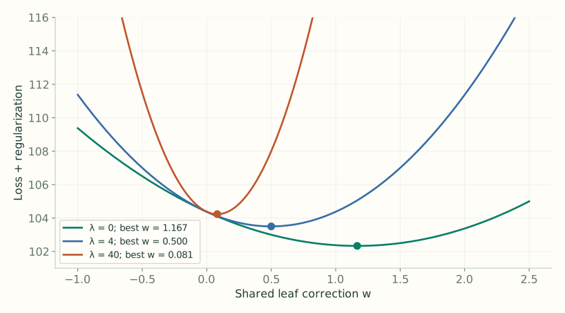
The full tree objective also charges $\gamma$ per leaf. While choosing the value of one existing leaf, its leaf count is fixed, so that charge does not affect the best $w$. It matters when comparing tree structures.

The penalty is on the leaf’s correction, not on the full current prediction $F_i+w$. Older contributions are not repeatedly shrunk by this new leaf’s penalty. We are controlling how aggressively this new tree changes the model.

For squared error, $\lambda$ has a particularly direct effect. If a leaf has $n$ rows with mean residual $\bar r$, its output is $n\bar r/(n+\lambda)$. Relative to the unregularized mean, the multiplier is $n/(n+\lambda)$. More rows reduce the relative shrinkage for the same $\lambda$.

Use the local slope and curvature for other losses

For a general loss, adding $w$ may not produce a simple quadratic. XGBoost uses a second-order Taylor approximation around the current prediction:

Here $g_i$ is the loss’s slope with respect to $F_i$, and $h_i$ is its second derivative, or curvature. The slope tells us which direction lowers the loss. Curvature tells us how quickly that slope changes as we move.

The first term is the old loss. It contains no $w$, so it cannot change which correction minimizes the expression. Add the remaining terms across the leaf, include regularization, and define $G=\sum g_i$ and $H=\sum h_i$:

Many rows have now become two totals: $G$ adds their slopes, and $H$ adds their curvatures. For squared error this quadratic is exact. For binary log loss it is a local approximation.

How the row terms become one leaf objective

For three rows in the same leaf, the linear terms are $g_1w+g_2w+g_3w$. Because the correction is shared, factor out $w$ to get $(g_1+g_2+g_3)w=Gw$. The quadratic terms combine in the same way to give $\frac12(h_1+h_2+h_3)w^2=\frac12Hw^2$.

The leaf penalty adds another $\frac12\lambda w^2$, producing $\frac12(H+\lambda)w^2$. The denominator $H+\lambda$ therefore consists of loss curvature from the data plus curvature from the penalty. It was not inserted merely to make the output smaller.

For a proposed feature split, change the row memberships and calculate these totals separately for each child. The derivatives themselves are still evaluated at the current model; they are not recalculated for every trial threshold.

Find the bottom of the quadratic

Differentiate with respect to the single correction $w$, and set the slope to zero:

When $H+\lambda>0$, the curve opens upward, so this stationary point is its minimum. If the combined slope is negative, the correction is positive; if the slope is positive, the correction is negative.

For the three-row example, $G=-3.5$ and $H=3$. With $\lambda=4$, the output is $3.5/7=0.5$. Learning rate is a separate step: at $\eta=0.3$, the ensemble actually adds $0.3(0.5)=0.15$.

A leaf is a compromise among its rows

If every row in a leaf asks for the same direction, its slopes reinforce one another. If some ask to go up and others down, they can cancel in $G$. A zero $G$ gives output zero even when individual rows have large errors. It means this group has no useful shared local correction, not that every row is already correct.

The second derivative of $Q$ is $H+\lambda$. A positive value makes the quadratic convex, which justifies taking its stationary point as the minimum. The squared-error and binary-log-loss examples supply nonnegative row curvatures; arbitrary custom losses need their own checks before applying this reasoning.

Plug in the loss to recover the first two videos

For regression, the minus sign in $-G$ turns the sum of negative residuals back into the sum of residuals. Adding one curvature value of 1 per row gives the row count.

For classification, derivatives are taken with respect to the log-odds score $F$, where $p=\operatorname{sigmoid}(F)$. Binary log loss can be written $\ell(y,F)=\log(1+e^F)-yF$. Its first derivative is $p-y$, and differentiating once more gives $p(1-p)$. That is why this denominator produces a score correction rather than a probability correction.

If you want every step of that conversion, the gradient boosting classification derivation covers it.

Evaluate the best correction to get the score

Finding $w^*$ tells us where the minimum is. Substituting it into $Q$ tells us how much the objective can improve:

The value is negative because this is the change relative to making no correction. A more negative value means a larger predicted loss reduction. Flip its sign to express an improvement; the lecture then uses twice that improvement as its similarity score:

Splitting replaces one optimized leaf with two optimized leaves. With this score convention, its gain is $S_L+S_R-S_P$.

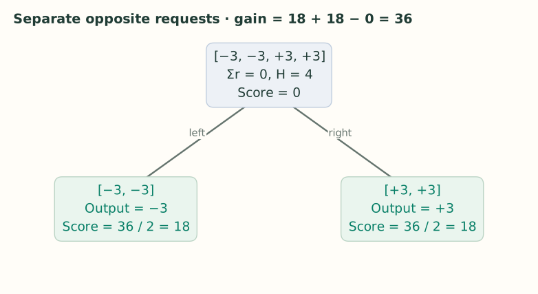
Where did the factor of ½ go? The paper writes the objective as $\sum\ell+\gamma_{\text{obj}}T+\frac{\lambda}{2}\sum_jw_j^2$. Under that definition, the benefit of adding one leaf through a split is

The videos use the unhalved score and compare its gain with a threshold on that same scale. XGBoost’s basic tree scorer also returns $G^2/(H+\lambda)$. Scaling every score preserves candidate rankings, but a pruning threshold must use the matching scale: threshold 10 on the unhalved gain corresponds to penalty 5 in the objective above.

This convention explains the apparent difference between the lecture’s arithmetic and the objective derivation in the documentation; it does not change the leaf output.

The optimized leaf scores compare whole structures

For a tree with leaves $1,\ldots,T$, every row belongs to one leaf. Add the optimized objective changes of those leaves and the leaf-count penalty:

This is an objective change after dropping terms common to all candidates, not the absolute training loss. For a fixed structure, its leaves can be optimized separately because changing one leaf’s output does not change the rows routed into the others.

A split replaces one parent leaf with two children, increasing $T$ by one. Subtracting the children’s optimized objective from the parent’s gives the reduction formula above. That is why the split comparison contains both the parent score and one extra leaf penalty.

Why splitting can have negative gain when λ is positive

Use the regression pair $[6.5,7.5]$ from Part 1 and set $\lambda=1$. Together, their score is $14^2/3\approx65.33$. Separate singleton leaves score $6.5^2/2=21.125$ and $7.5^2/2=28.125$.

The two rows already want nearly the same correction. Creating two regularized leaf outputs buys little extra fit and incurs separate leaf penalties. The regularized score can therefore prefer keeping them together even when the leaf-count threshold is zero.

Without regularization, the two singleton leaves can at least reproduce any output available to the shared leaf, so their optimized unpenalized fit cannot be worse. With leaf penalties, changing the number of leaf outputs changes the optimization problem.

Cover is the total curvature we already calculated

Cover is simply $H=\sum h_i$. For unweighted squared-error regression, it equals the row count. For binary classification, it equals $\sum p_i(1-p_i)$.

We now have the whole connection: the loss supplies slopes and curvatures; their totals give a leaf correction; evaluating that correction gives a score; comparing parent and child scores chooses a feature split. The new tree then supplies the scaled corrections used by the ensemble.

Finally, a split score estimates training-objective improvement for a proposed correction tree. It does not estimate validation AUC, test error, or the causal importance of a feature. Those are separate questions requiring the corresponding evaluation data or assumptions.