2. Classification: From Corrections to Probabilities
Notes on StatQuest with Josh Starmer · Classification: From Corrections to Probabilities · 25:17 video. Original explanations and redrawn figures accompany the video.
The tree still predicts a correction. For binary classification, however, we add that correction to a log-odds score, then convert the result into a probability.
Two scales: score and probability
Video 1:57 ↗The outcome is whether a drug is effective: $y=1$ for yes, $y=0$ for no. Start every row at probability $p=0.5$, corresponding to score $F=0$:
A positive score means probability above 0.5; a negative score means below 0.5. These are two representations of the same prediction.
| Dosage | Outcome $y$ | Current $p$ | Residual $r=y-p$ | Curvature $h=p(1-p)$ |
|---|---|---|---|---|
| 2 | 0 | 0.5 | −0.5 | 0.25 |
| 8 | 1 | 0.5 | 0.5 | 0.25 |
| 12 | 1 | 0.5 | 0.5 | 0.25 |
| 18 | 0 | 0.5 | −0.5 | 0.25 |
Residual signs tell us the desired direction: lower the prediction for rows with outcome 0, raise it for rows with outcome 1. The curvature will help determine the size of the score correction.
The labels are binary; the tree outputs are numeric
The final classifier returns a probability of outcome 1. Each tree is a component of that classifier, and its job is to change a numeric score. Its leaves therefore store positive or negative numbers, not just class labels.
The first two positive residuals do not mean the tree should add 0.5 to the probability. They mean the current model assigns too little probability to the observed outcome 1. XGBoost uses those requests together with curvature to choose a correction on the score scale.
The score changes its denominator
Video 3:21 ↗Classification uses
Regression counted rows in the denominator. Classification instead adds their $p_i(1-p_i)$ values. For now each row contributes 0.25, and we set $\lambda=0$.
All four residuals sum to zero, so the root score is zero. One shared update would cancel the positive and negative requests.
The denominator is evaluated using the current model, before adding this tree. A node containing three of these rows has curvature total $3(0.25)=0.75$. A singleton has 0.25. We calculate these totals for each candidate child, just as regression counted the rows in each child.
Using the sum of curvatures is what makes the same tree-building machinery work with binary log loss. The feature threshold still determines membership; the score evaluates how useful a shared correction would be for those members.
Separate the requests to raise and lower the score
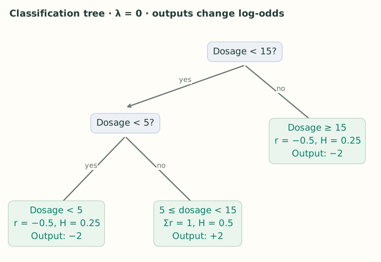
Video 5:44 ↗The lecture chooses dosage $<15$ for the first split. Its left child contains $[-0.5,0.5,0.5]$, while the right contains $[-0.5]$.
The gain is $1/3+1-0=4/3\approx1.33$. Splitting at 5 ties this gain; 15 is the choice shown in the video. A tie does not identify a unique tree.
Now split the left child at 5. This separates $[-0.5]$ from $[0.5,0.5]$:
The alternative threshold 10 gives only $2/3\approx0.67$. The selected tree has three leaves, each containing residuals that agree on the direction of correction.
| Threshold | Left residual sum / cover | Right residual sum / cover | Gain |
|---|---|---|---|
| 5 | −0.5 / 0.25 | +0.5 / 0.75 | 4/3 |
| 10 | 0 / 0.50 | 0 / 0.50 | 0 |
| 15 | +0.5 / 0.75 | −0.5 / 0.25 | 4/3 |
At threshold 10, each child contains one negative and one positive residual. Their requests cancel, so neither child has a useful shared score correction in this round. The two outer thresholds begin to separate the negative cases from the positive cases.
Cover measures the curvature in a child
Video 9:49 ↗Cover is $H=\sum p_i(1-p_i)$. It excludes $\lambda$. The two singleton leaves above each have cover 0.25; the two-row leaf has cover 0.50.
min_child_weight sets the minimum permitted child cover. With a threshold of 1, none of these tiny leaves qualifies. The lecture relaxes this constraint to build its example; set it explicitly to 0 when reproducing the tree.
Why not just count rows? At $p=0.5$, a row contributes 0.25. At $p=0.99$, it contributes only 0.0099. The same number of rows can therefore have very different cover as predictions change. This constraint is about curvature support, not a fixed row count.
Why the default child-cover constraint blocks this tiny example
At $p=0.5$, four equally weighted rows are needed to reach cover 1. A valid split with minimum child cover 1 would need at least four such rows on each side. Our entire dataset has only four, so even the first split cannot pass.
This is separate from whether the gain is high. A candidate can improve the objective yet be rejected because one child lacks enough curvature support. Setting min_child_weight=0 removes that particular barrier for the teaching example.
Pruning uses the same bottom-up idea
Video 13:05 ↗Using the lecture’s gains, $\gamma=2$ keeps the lower split because $2.67>2$. The root remains because it leads to that subtree. At $\gamma=3$, the lower split fails; after removing it, the root’s gain of 1.33 also fails.
In this particular first-round example, the remaining root leaf has output zero because the residuals sum to zero. That is why a fully collapsed tree makes no change here.
Calculate the amount to add to the score
Video 14:58 ↗The leaf output is
With $\lambda=0$, a negative singleton produces $-0.5/0.25=-2$. The middle pair produces $1/0.5=2$. Unlike regression, simply averaging residuals would not give these outputs.
The denominator converts a loss-reducing direction into a step on the log-odds scale. The next note derives it from binary log loss. For now, keep the scales straight: $y-p$ measures what is wrong with the current probability; $w$ is the correction we add to the score.
Regularization shrinks this correction. With $\lambda=1$, the singleton becomes $-0.5/1.25=-0.4$, while the positive pair becomes $1/1.5\approx0.667$.
Why divide by curvature rather than just average the residuals?
For a positive singleton at $p=0.5$, the residual is 0.5 but the Newton score step is $0.5/0.25=2$. Near the current score, the slope of log loss changes at rate 0.25. Dividing the desired negative slope by that rate estimates how far to move the score before the slope reaches zero.
It is a local estimate, not an exact correction that makes the probability equal the label. Even adding the full score step 2 to 0 gives sigmoid probability about 0.881, not 1. The learning rate of 0.3 makes the actual first step smaller still.
A very confident prediction has low curvature. If a single row has $y=0$ but $p=0.99$, the unregularized step is $-0.99/0.0099=-100$. With $\lambda=1$, it becomes about −0.9803. This illustrates why a small denominator can produce an extreme local step, and how regularization stabilizes it.
Update the score, then apply sigmoid
Video 17:26 ↗Return to $\lambda=0$ and use learning rate $\eta=0.3$. Dosage 8 reaches the positive leaf:
Dosage 2 reaches a negative leaf, so its score becomes −0.6 and its probability becomes about 0.354. Both predictions move toward their observed labels.
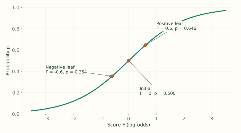
Adding 0.6 directly to probability 0.5 would give 1.1. That invalid result is precisely why we do the addition on the score scale.
Refresh both residuals and curvature
Video 22:02 ↗Before the next tree, recompute $r_i=y_i-p_i$ and $h_i=p_i(1-p_i)$ using the new probabilities.
| Rows | New probability | New residual | New curvature |
|---|---|---|---|
| Dosages 2 and 18; $y=0$ | 0.3543 | −0.3543 | 0.2288 |
| Dosages 8 and 12; $y=1$ | 0.6457 | 0.3543 | 0.2288 |
The curvature happens to match across these symmetric probabilities. In general it differs by row. Build the next tree from these updated quantities, add its scaled output to $F$, and convert to probabilities again.
Calculate a second update with the same three regions
For the positive pair after tree 1, each row has $r\approx0.3543$ and $h\approx0.2288$. Their combined leaf output is
For either negative singleton the output is −1.5488. The second tree’s values are smaller than the first tree’s ±2 because the updated model is already closer to the observed labels.
| Rows | Initial p | After tree 1 | After tree 2 |
|---|---|---|---|
| Dosages 8 and 12; y = 1 | 0.5000 | 0.6457 | 0.7436 |
| Dosages 2 and 18; y = 0 | 0.5000 | 0.3543 | 0.2564 |
The positive score becomes $0.6+0.3(1.5488\ldots)=1.0646\ldots$, which sigmoid converts to 0.7436. Reusing the old leaf output +2 would give a different result because it would ignore the refreshed residuals and curvatures.
For a new dosage of 9, both of these example trees select the positive middle leaf. The model needs that dosage to select the saved corrections; it does not need to know whether the drug actually worked for this new case.