4. Optimizations: Search Less, Move Data Faster
Notes on StatQuest with Josh Starmer · Optimizations: Search Less, Move Data Faster · 24:27 video. Original explanations and redrawn figures accompany the video.
The first three lectures explain what XGBoost calculates. This lecture explains how it avoids doing unnecessary work when there are many rows and features.
Greedy search still has many candidates
Video 1:34 ↗At a node, XGBoost scores candidate feature thresholds and chooses the best available split. “Greedy” means it makes that local choice without exploring every possible future tree below each candidate.
Even this can be expensive. A continuous feature with a million distinct values has nearly a million possible boundaries. Repeating a full scan across many features and nodes costs time.
Even an exact scan can reuse its work
After sorting rows by one feature, move a candidate boundary from left to right. When it passes a row, add that row’s gradient and Hessian to the left totals. The right totals are the parent totals minus the left totals. We do not need to sum every child from scratch at each boundary.
For the regression example in Part 1, gradients are the negatives of the residuals: $[10.5,-6.5,-7.5,7.5]$, with Hessian 1 for each row. The parent totals are $G_P=4$ and $H_P=4$.
| Threshold | $G_L$ | $H_L$ | $G_R$ | $H_R$ | Gain |
|---|---|---|---|---|---|
| 15 | 10.5 | 1 | −6.5 | 3 | 120.33 |
| 22.5 | 4.0 | 2 | 0.0 | 2 | 4.00 |
| 30 | −3.5 | 3 | 7.5 | 1 | 56.33 |
For example, advancing from 15 to 22.5 moves the dosage-20 row left. Its gradient −6.5 changes $G_L$ from 10.5 to 4, and its Hessian 1 changes $H_L$ from 1 to 2. The same gain formula can then evaluate the new boundary immediately.
Approximate search considers fewer boundaries
Video 3:59 ↗Instead of testing every boundary, choose a smaller set of candidate cuts. Quantiles put those cuts where the data lies, rather than wasting equal-width intervals on nearly empty ranges.
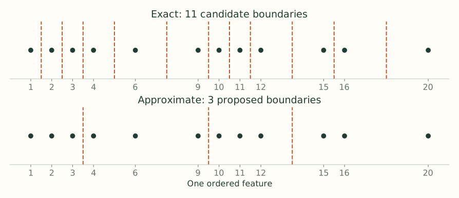
For each candidate, the scoring rule stays the same: collect left and right gradient and curvature totals, then calculate gain. Approximation changes which splits are considered, not the meaning of gain.
More bins give the search finer resolution and more work. They do not guarantee better validation performance. A cut can only separate values lying on opposite sides of an available boundary.
See the cost of a coarse bin in the original example
Suppose binning leaves only the boundary at 22.5 between the two pairs of dosages. That scan can obtain gain 4, but it cannot consider the exact scan’s winning boundary at 15 with gain 120.33. The useful separation lies inside the first bin.
This is what approximation can lose. The scoring formula is still correct for the boundaries it tests; the missing option is a better boundary. More resolution can make that option available, at the cost of larger summaries and more candidate evaluations.
The word “exact” refers to the candidate threshold search, not to a globally optimal tree. An exact greedy scan can still choose a root that would lose to another root after looking several levels ahead.
Summarize pieces of the data and merge the summaries
Video 6:40 ↗To get candidate quantiles from a large dataset, XGBoost need not send every sorted value to one machine. Workers can summarize their local data with a quantile sketch, and those summaries can be merged into an approximate summary of the whole feature.
The worker summaries preserve approximate information about where ranks fall. They are not independent trees whose predictions get averaged. Work inside tree construction can run in parallel; the next boosting round still depends on the predictions produced by preceding rounds.
A quantile sketch and a node histogram have different jobs
The sketch helps propose boundaries from feature values and weights. After boundaries are chosen, a node’s histogram records gradient and Hessian totals in those bins for the rows reaching that node. Cumulative histogram sums then provide the left and right statistics needed for gain.
Workers can accumulate their own bin totals and add them to obtain totals for the combined data. Adding sums is much cheaper than repeatedly exchanging every underlying row. The training objective still uses the combined statistics; each worker is not solving an unrelated prediction task.
Weighted quantiles allocate resolution by curvature
Video 8:03 ↗Ordinary quantile bins aim for similar row counts. The lecture’s weighted quantiles aim for similar total weight, using each row’s Hessian $h_i$ as its weight.
For unweighted squared-error regression, every $h_i=1$, so weighting reduces to ordinary counts. For binary log loss, $h_i=p_i(1-p_i)$. The lecture uses six ordered observations with the following current probabilities:
| Ordered row | Current $p$ | Weight $p(1-p)$ |
|---|---|---|
| 1 | 0.1 | 0.09 |
| 2 | 0.1 | 0.09 |
| 3 | 0.9 | 0.09 |
| 4 | 0.9 | 0.09 |
| 5 | 0.6 | 0.24 |
| 6 | 0.4 | 0.24 |
The first two weights add to 0.18, as do the next two. Each of the last rows already carries 0.24. The video illustrates bins $[1,2]$, $[3,4]$, $[5]$, $[6]$: similar weight totals, despite different row counts.
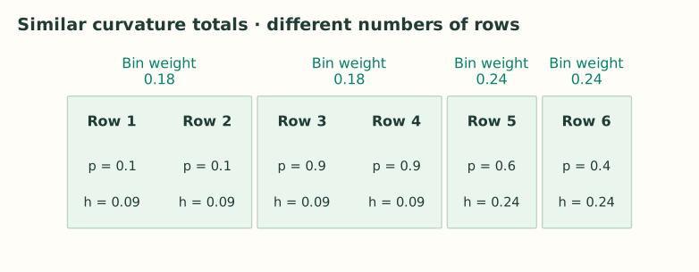
Why does that help? If two rows need opposite corrections but fall in the same bin, the search cannot separate them using this feature. Finer bins near uncertain probabilities can make that separation available. This is curvature weighting, not “give every mistake more weight”: a confidently wrong prediction can still have small $p(1-p)$.
Current API distinction: tree_method="approx" uses Hessian-weighted sketching before each tree. "hist" uses a global sketch based on user-supplied row weights, then accumulates gradients and Hessians in those bins. The lecture’s sketch explanation should not be read as the exact procedure for every tree method. See Tree Methods.
Why the weighted bins have unequal numbers of rows
The six curvature weights total 0.84. Dividing that mass into four equal portions would target 0.21 per portion. Two low-curvature rows together contribute 0.18, close to that target; one high-curvature row contributes 0.24, also close. Two high-curvature rows together would contribute 0.48 and occupy too much of the budget in one bin.
The illustrated grouping is therefore understandable without the internal sketch algorithm. Its purpose is to show why one bin might hold two rows while another holds one. The lecture’s ordinary and weighted pictures are illustrations, not a proof that a fixed bin budget always separates every difficult pair.
At the initial probability 0.5, all rows have the same Hessian, so Hessian weighting cannot yet distinguish them. The unequal weights arise after previous trees have produced different probabilities. This is why an algorithm using fresh Hessian-weighted sketches may revise its proposed boundaries between rounds.
Learn which branch missing values should take
Video 16:13 ↗Suppose dosage is missing for some rows, but their target values are known. They still have residuals; we just cannot order them by dosage. For each proposed threshold, try sending all rows missing that feature left, then try sending them right. Keep the better gain and store its direction.
The lecture’s known dosages are $[5,10,21,25]$, with residuals $[-5.5,-7.5,6.5,7.5]$. Two rows have missing dosage and residuals $[-3.5,-2.5]$. Use $\lambda=0$.
At threshold 15.5, the known rows split into negative and positive corrections. The parent has residual sum −5 across six rows, so its score is $25/6$. Sending the missing rows left gives
Sending them right instead gives
| Threshold | Missing left: gain | Missing right: gain |
|---|---|---|
| 7.5 | 54.00 | 26.13 |
| 15.5 | 184.08 | 96.33 |
| 23 | 83.33 | 10.67 |
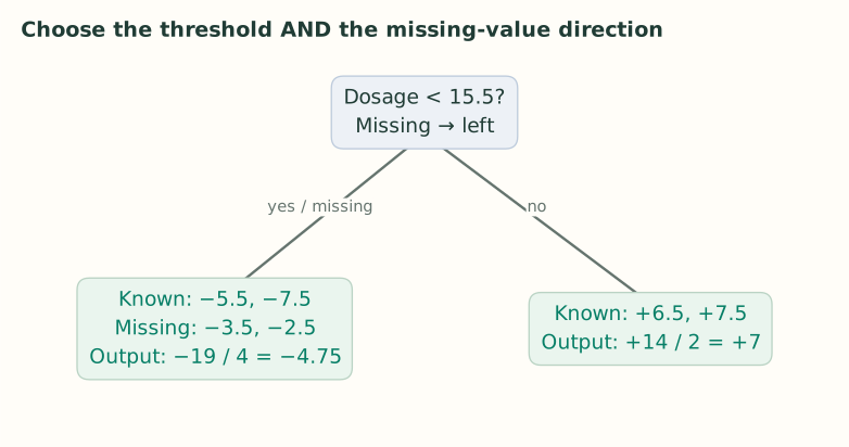
The winning choice is threshold 15.5 with missing values sent left. Another node or feature may learn a different default. The model has learned a route, not an imputed numeric dosage.
With dense Python arrays, use np.nan for missing values. Zero is an ordinary observed value unless you explicitly designate it as missing. Sparse omitted entries have different semantics for tree boosters; see the XGBoost FAQ.
The missing rows still contribute to the objective
We set aside the missing feature values while ordering the known values; we do not discard those rows from the gain calculation. Their gradients and Hessians must be included on whichever side is being tested. The parent statistics always include both known and missing rows.
At prediction time, a row with observed dosage 12 follows the ordinary threshold comparison. A row with missing dosage follows the stored default direction instead. Both can reach the same leaf, but by different routing rules.
“Missing” is specific to the feature used at the current node. If a later node tests a different, observed feature, that row can use a normal threshold comparison there. It is not assigned one global missing-data branch for the entire ensemble.
Keep the scoring loop supplied with data
Video 20:34 ↗Arithmetic is only part of runtime. A processor can spend much of its time waiting for the needed gradients, Hessians, and feature values.
| Optimization | What it saves |
|---|---|
| Cache-aware access | Arrange access and buffer gradient statistics so the inner scoring loop waits less on slower memory. |
| Reusable sorted blocks | Organize feature data for repeated scans instead of repeatedly sorting everything from scratch. |
| Out-of-core blocks | Stream manageable blocks when the whole dataset does not fit in main memory. |
| Compression and prefetching | Read fewer bytes and prepare the next block while computation processes the current one. |
| Sharding across disks | Read different data blocks concurrently where the storage system supports it. |
These mechanisms are described in the original XGBoost paper, especially Sections 4 and 5. They improve data access around the same gradient and Hessian calculations.
Sorting a feature orders the feature values, but it can leave the corresponding gradient records scattered in memory. Fast arithmetic does not help if each lookup waits on a slow memory access. Cache-aware buffers and access patterns reduce that waiting by bringing useful statistics closer to the scoring loop.
Out-of-core training addresses a larger limit: the data exceeds main memory. Streaming compressed blocks avoids requiring the entire dataset to be resident at once. Decompression consumes CPU time, but it can be worthwhile when reading fewer bytes saves more time than decompression costs.
Use fewer rows or features per tree
Video 23:11 ↗The lecture ends with two more ways to reduce work: sample rows and sample features. In the Python API, subsample controls the row fraction and colsample_bytree controls the feature fraction for each tree.
Sampling also changes the fitted model and can reduce overfitting, so choose these settings using validation results. Across all these optimizations, keep track of what changed: the available candidates, the data used for a tree, or the cost of moving the same data through the computer.