Prediction Losses & Best ConstantsOverview

Prediction Losses and Their Best Constants

September 2026 · 5 min read + loss explorer

Before a model learns anything about the input features, what should it predict for every row? The answer depends on the loss: the same observations can favor a mean, a median, a probability, or a balance of clipped residuals.

What “best constant” means

Take $n>0$ training observations and make the raw score the same number $c$ for all of them. We choose that number by minimizing the total training loss:

$$J(c)=\sum_{i=1}^n\ell(y_i,c),\qquad c^*\in\arg\min_c J(c).$$

This is a one-parameter optimization problem. There are no feature weights or splits yet. In gradient boosting, $F_0(x)=c^*$ is the starting score; later trees add corrections that depend on $x$. The reported prediction may be $c$ itself, a probability $\sigma(c)$, or a mean count $e^c$.

Every derivation below uses equally weighted training rows and no penalty on the constant. Dividing $J$ by $n$ changes its scale, but not its minimizers.

The results, with the derivation one click away

Loss	Reported constant prediction	Best raw score $c^*$
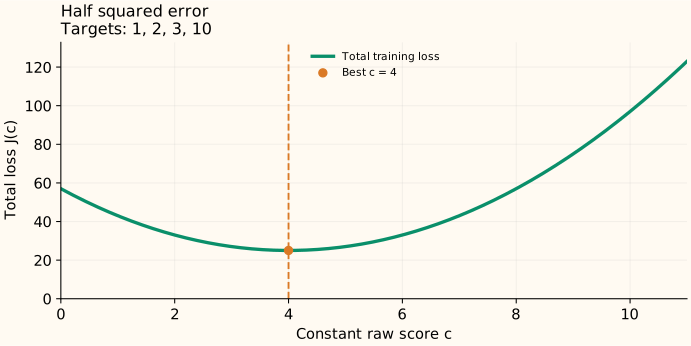
Half squared error	Mean target	$\bar y$
Absolute error	Any empirical median	A median of the targets
Binary log loss	Positive-label fraction $\bar y$	$\log\!\frac{\bar y}{1-\bar y}$ when $0<\bar y<1$
Poisson loss, equal exposure	Mean count $\bar y$	$\log\bar y$ when $\bar y>0$
Huber loss, fixed $\delta$	A balance of capped errors	A root of $\sum_i\operatorname{clip}(c-y_i,-\delta,\delta)=0$

Binary data containing only one class and Poisson data containing only zeros have boundary optima: the best reported prediction exists, but no finite log-odds or log-mean score represents it. The individual pages explain those cases.

Move the constant and inspect the actual objective

Choose a loss, then move $c$. The curve is the sum of that loss over the displayed targets. Its minimum is marked separately from your chosen score. Absolute error has a whole interval of equally good answers in this example; that flat segment is part of the result.

Total training loss against a shared constant score, with the minimizing score or interval marked. The targets and numerical optimum are stated in the text. — The curve sums the stated loss over all displayed observations. The orange mark shows the minimizing score or interval; the blue point follows your chosen constant. Open the computed figure.

Read the five derivations

Squared error: summing residuals gives the mean.
Absolute error: counting observations on each side gives a median.
Binary log loss: match the class fraction, then convert probability to log odds.
Poisson loss: match the mean count, then convert it to a log mean.
Huber loss: balance residuals after clipping their influence.

Starting a model versus fitting its next tree

The starting constant uses the original targets. A later tree fits corrections to the current model. The StatQuest regression example shows how feature thresholds group rows whose pseudo-residuals can share a correction.

The other branches of the loss-functions series study entropy, distribution divergences, transport, and triplet objectives. Those do not all optimize a scalar prediction against an observed target, so the constant-score formulas here should not be applied to them automatically.

Sources and reproducible figures

The examples and plots are computed by this reproduction script, which also checks the stated minima. Inspect the figure data.