Naïve Bayes: From Probability Models to Classification
Following Naïve bayes.pdf, pages 1–8 · View a handwritten page
The notes begin with fitting probability distributions, then use Bayes' rule to turn them into a classifier. We will follow that sequence: estimation, conditional independence, the three feature models, and the connection to a linear decision rule.
First, fit a probability model
We do not know the distribution that generated our data. We choose a family of distributions and estimate its parameters $\theta$ from the training data $D$.
Maximum likelihood (MLE) chooses the parameters under which the observed data have the greatest likelihood:
Maximum a posteriori (MAP) also uses a prior over the parameters:
Both give one fitted model, which predicts using $P(y\mid x,\hat\theta)$. The notes also show Bayesian prediction: average the predictions of possible models, weighted by their posterior probabilities.
Why use Bayes' rule for classification?
We want $P(y\mid x)$: the probability of a label after observing an input. Write the input as $x=(x_1,\ldots,x_d)$, with $d$ features. Counting how often each complete input occurs becomes unreliable in many dimensions: most combinations have few or no matching training rows.
The notes reverse the problem. Estimate how common each class is and how inputs occur within it. For a candidate class $c$, Bayes' rule gives:
The numerator combines how well the input fits the class with how common that class is. Here $P(c)$ is a class prior; it is different from the parameter prior $P(\theta)$ used in MAP. The denominator $P(x)$ is the overall probability of the input, allowing for every class.
Expand the denominator
If the only classes are spam ($S$) and non-spam ($H$), the input must arrive with one of those two labels. The possibilities do not overlap, so their probabilities add:
For any number of classes, sum over all labels $k$. Substituting this sum into Bayes' rule gives:
This denominator makes the class probabilities sum to one. It is the same for every candidate class, so choosing the largest posterior only requires comparing the numerators.
Make the class-conditional model manageable
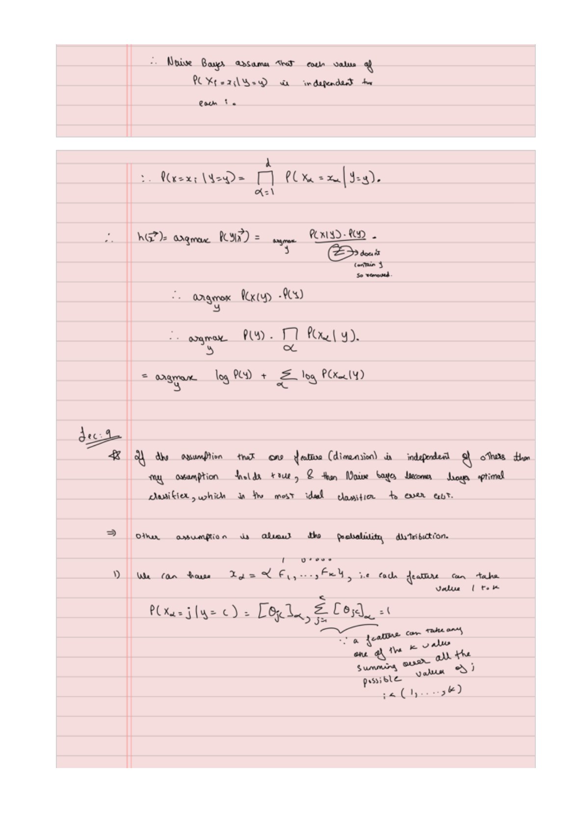
Reversing the probability has not yet solved the problem: $P(x\mid c)$ still describes a whole feature combination. The naïve assumption is that features are independent once the class is known:
The index $\alpha$ picks a feature, and $\prod$ means multiply. We now estimate one small distribution per feature and class, then multiply their values. Independence is assumed within each class, not across the entire dataset.
Substitute this product into the decision rule. Here $\arg\max$ means “choose the class giving the largest value”:
Turn products into log scores
Logarithms preserve which positive value is largest and turn multiplication into addition. They also prevent long products of small probabilities from underflowing on a computer.
If conditional independence holds and we know the correct class and feature distributions, this is the Bayes-optimal classifier: it minimizes the probability of a wrong label when all classification errors have equal cost. Estimated probabilities and imperfect assumptions can change that result.
Choose a distribution for each kind of input
Independence tells us how to combine features. We still need a model for their values. The notes consider categorical values, word counts, and continuous measurements, in that order.
Categorical: one value from a set
Suppose feature $\alpha$ can take one of $K_\alpha$ categories. For each class, give those categories their own probabilities:
$\theta_{jc}^{(\alpha)}$ is the probability of category $j$ for feature $\alpha$ in class $c$. The probabilities sum to one because the feature must take one of its possible values. Estimate a category's probability by its frequency among training rows of that class. Each feature has a separate probability table for each class.
Multinomial: count occurrences of words
The model keeps how many times each word appears and discards word order. We want the probability of getting those counts, given a message length $m$ and a candidate class $c$.
Build the probability of a count vector
Keep one message in mind: “free free prize.” Suppose our vocabulary contains three words and class $c$ has the following word probabilities:
| Word | Probability on each draw | Count in message |
|---|---|---|
| free | 0.5 | 2 |
| prize | 0.3 | 1 |
| meeting | 0.2 | 0 |
The probabilities sum to 1 because each draw produces one vocabulary word. The counts are $x=(2,1,0)$ and the length is $m=3$. Read $P(x\mid m,c)$ as: “Using class c's word probabilities, how likely are we to get these counts in three draws?”
1. Find the probability of one exact order. The model draws each word independently using the same probabilities. To get free, then free, then prize, multiply:
We can write this as $0.5^2\times0.3^1\times0.2^0$. The exponent is the number of occurrences: two “free” draws, one “prize” draw, and no “meeting” draws. A zero exponent contributes a factor of 1.
2. Include every order with those counts. The count vector $(2,1,0)$ represents all three of these sequences:
- free, free, prize
- free, prize, free
- prize, free, free
Each sequence has probability 0.075: rearranging the same three factors does not change their product. The sequences are separate possible outcomes, so we add their probabilities:
Under this class model, a three-word message has a 22.5% chance of containing exactly two “free” words and one “prize,” in any order.
3. Count the orders without listing them. The factorial $3!=3\times2\times1=6$ counts arrangements of three distinguishable items. Imagine temporarily labeling our two copies “free₁” and “free₂.” Swapping those copies creates a different labeled arrangement, but the same visible words. Every visible sequence was therefore counted twice, so divide by $2!=2$:
The one copy of “prize” contributes $1!=1$ to the denominator; the zero copies of “meeting” contribute $0!=1$. Neither changes the result.
Now write the same calculation for any message. The vocabulary has $d$ words, indexed by $\alpha$. The count of word $\alpha$ is $x_\alpha$, and its probability in class $c$ is $\theta_{\alpha c}$. For “free,” $x_1=2$ and $\theta_{1c}=0.5$. The message length is $m=\sum_{\alpha=1}^{d}x_\alpha$.
The symbol $\prod$ means multiply over all vocabulary words. Thus $\prod_\alpha x_\alpha!$ means $x_1!\times\cdots\times x_d!$, and $\prod_\alpha\theta_{\alpha c}^{x_\alpha}$ repeats each word's probability according to its count:
In our message, those two factors are 3 and 0.075—the same calculation we already made. For a given message, the order-counting factor is the same for every class, so it cancels when comparing classes. The word probabilities are what change.
We treat the length $m$ as given, without fitting a separate length distribution. The independent draws produce counts that must sum to $m$; the counts themselves are not independent.
Estimate the word probabilities from training data
Now use $n$ for the number of training messages. Message $i$ has label $y_i$, word counts $x_{i\alpha}$, and length $m_i$. The indicator $I(y_i=c)$ is 1 when the message belongs to class $c$ and 0 otherwise: it selects only that class's rows.
The MLE in the notes is:
The numerator counts occurrences of this word in class $c$. The denominator counts all words in that class. The index $\beta$ above runs through the vocabulary to calculate each message's length.
The class prior uses a different count: the number of messages in the class, divided by the total number of messages.
Why add one upstairs and d downstairs?
If a word never appeared in a class, its MLE probability is zero. Any new message containing it would then get zero likelihood for that class. Laplace smoothing adds one count to every vocabulary word:
There are $d$ words, so adding one to each adds $d$ to the total. This keeps the probabilities positive and makes them sum to one. The extra $d$ counts are word occurrences, not extra training messages.
Classify by comparing posterior odds
The word count $x_\alpha$ first appears as an exponent in the likelihood: a word occurring $x_\alpha$ times contributes $\theta_{\alpha c}^{x_\alpha}$. Using the fitted probabilities and dropping the factorial factor shared by all classes, the score before taking logs is:
Taking a log turns the product into a sum. Then the rule $\log(a^b)=b\log a$ brings each word count down from the exponent:
So $x_\alpha$ tells us how many times to add that word's log probability. In “free free prize,” “free” occurs twice: $\log(\theta_{1c}^2)=2\log\theta_{1c}$. “Prize” contributes once, and the absent “meeting” contributes zero.
For two classes, the notes express the decision as a ratio. Bayes' common denominator cancels:
A ratio above 1 favors spam; below 1 favors non-spam; exactly 1 is a tie. Equivalently, choose the larger log score. From here onward, the probabilities and parameters refer to their fitted values, so we omit the hats.
Gaussian: model continuous features
For a real-valued feature, the notes assume a Gaussian distribution with a separate mean and variance for each feature and class:
Its density at the observed value is:
$\mu_{\alpha c}$ sets the center and $\sigma_{\alpha c}^2$ sets the spread. Values farther from the class mean have lower density. For continuous inputs these are densities, rather than probabilities of exact values; Bayes' rule combines them in the same way.
Fit the mean and variance within each class
Using the same class selector and row count $n_c$, the MLEs are:
First average the feature values in class $c$. Then average their squared distances from that mean. The variance divides by $n_c$ because this is the maximum-likelihood estimate, not the unbiased sample-variance estimate. Multiply the fitted feature densities and the class prior to obtain each class's score.
Why can a perceptron separate points that Naïve Bayes misses?
The notes compare two ways to learn a classifier. A perceptron directly adjusts a separating hyperplane in response to classification mistakes. Naïve Bayes fits class distributions and obtains its boundary from those distributions.
On a finite, linearly separable training set, the standard perceptron algorithm finds a separator after finitely many updates. Naïve Bayes has no such training-set guarantee: a poor distributional assumption can put its boundary in the wrong place even when a separating line exists.
When the data are not linearly separable, the standard perceptron has no convergence guarantee. Naïve Bayes can still fit distributions and make predictions, but non-separability alone does not make it the better model. Performance on unseen data is a separate question for both.
Derive the linear decision rule
The notes next use labels $+1$ and $-1$ for the two classes. Write their priors as $\pi_+$ and $\pi_-$. For a multinomial model, the positive class wins when its prior times its likelihood is larger. Cancel the shared factorial factor, then take logarithms:
Move the negative-class terms to the left and combine each pair of logarithms into a log ratio:
The class-prior ratio supplies an intercept; each word-probability ratio supplies a weight:
This is a linear classifier in the word counts. A positive weight moves the decision toward the positive class whenever that word occurs. The boundary $w^\top x+b=0$ is where the two posteriors are equal.
When is the Gaussian boundary linear?
Gaussian log densities contain $(x_\alpha-\mu_{\alpha c})^2$. If a feature has the same variance in both classes, its $x_\alpha^2$ terms cancel when we subtract the two log scores. If this holds for every feature, the log odds are linear in $x$.
With different class variances, squared terms generally remain. This explains the notes' broader “linear in feature space” remark: exponential-family models with a shared base measure give log odds linear in their sufficient statistics—the input quantities used by the model. For Gaussians, those quantities can include both $x_\alpha$ and $x_\alpha^2$, so linearity in that expanded space need not mean a straight boundary in the original inputs.
Turn the log odds into the final probability
The last page gives a sigmoid expression. Let $g(x)$ denote the log posterior odds:
The odds are therefore $e^{g(x)}$. Since the two class probabilities sum to one, solving for the positive-class probability gives:
When the log odds are linear, $g(x)=w^\top x+b$. Both labels can then be written in the notes' compact form:
The bias $b$ can also be included in $w^\top x$ by adding a constant feature equal to 1. This is the same probability form used by logistic regression. Naïve Bayes obtains its weights from fitted class distributions; logistic regression fits the conditional class probabilities directly.
From the handwritten notes
This guide follows all eight pages of Naïve bayes.pdf: estimation and priors (1–2), conditional independence and the feature models (3–6), and perceptron comparison, linear classification, and the sigmoid (6–8).
View original page 3
References for the distribution formulas and classification conditions: