Entropy, Gini & Information Gain
The scan asks how a tree can choose between possible splits. Follow one eight-row example from class counts to entropy, then from child entropies to information gain. The purpose of a split is to leave less uncertainty about the label after we know which child a row enters.
Turn class proportions into uncertainty
A node containing only A has no training-label uncertainty. An equal mix of A and B has more. Let $p_k$ be the fraction of rows belonging to class $k$. Using base-2 logarithms, entropy is measured in bits:
An absent class contributes zero, using the limiting value of $-p\log_2 p$ as $p$ approaches zero. An equal two-class mixture gives 1 bit; a pure node gives 0. These values describe the observed class proportions, not the tree’s accuracy on unseen rows.
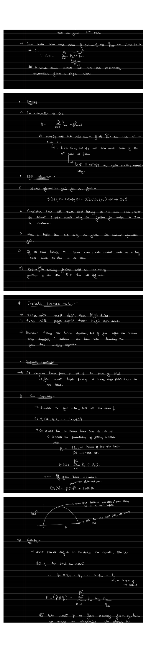
Our companion example has one numeric feature, x = 1 through 8, and ordered labels A, A, B, A, B, B, B, B. Each row has equal weight. Three of the eight labels are A, so the parent proportions are 3/8 and 5/8.
Parent entropy: −(3/8) log₂(3/8) − (5/8) log₂(5/8) ≈ 0.954434 bits.
The two terms contribute about 0.530639 and 0.423795 bits. Add them once for the whole parent; this value stays fixed while we compare its candidate splits.
A second way to measure the same mixture
Gini impurity is $G=1-\sum_k p_k^2$. It is the probability that two labels drawn independently from the node’s class distribution disagree. For the same parent, G = 1 − (3/8)² − (5/8)² = 0.46875. A balanced binary node has Gini 0.5; a pure node has Gini 0.
Entropy and Gini are different criteria with different scales; Gini is not measured in bits. Both reward concentrated child labels, but their preferred splits can differ. The example below uses entropy throughout. The worked impurity chapter compares the criteria more fully.
Weight each child by the rows that reach it
Use the rule x < t → left; x ≥ t → right. At threshold t = 4.5, the left child contains A, A, B, A and the right contains B, B, B, B. Each child receives four of the parent’s eight rows.
The left child’s own proportions are 3/4 and 1/4, giving entropy 0.811278 bits. The right child is pure, so its entropy is zero. To find the uncertainty remaining for a randomly selected parent row, weight those entropies by the chance of entering each child:
Remaining entropy:
(4/8) × 0.811278 + (4/8) × 0 ≈ 0.405639 bits.
Information gain:
0.954434 − 0.405639 ≈ 0.548795 bits.
The two fractions have different jobs: 3/4 describes the label mix within the left child; 4/8 describes how much of the parent reaches it. An unweighted average of child entropies happens to work for this equal-size split, but fails when child sizes differ.
Seven candidate cuts, one fixed parent
Each chip shows a feature value and its class. The child panels show the actual partition; the bars share a 0–1 bit scale. Compare the blue and amber contributions with the parent, then read their reduction as information gain.
Unsplit parent: 3 A, 5 B
- x=1A
- x=2A
- x=3B
- x=4A
- x=5B
- x=6B
- x=7B
- x=8B
Parent entropy: 0.954434 bits · 8 rows
Left: x < 4.5
- x=1A
- x=2A
- x=3B
- x=4A
- Class counts
- 3 A, 1 B · 4 rows
- Entropy within this child
- H(left) = 0.811278 bits
- Weighted contribution
- (4/8) × 0.811278 = 0.405639 bits
Right: x ≥ 4.5
- x=5B
- x=6B
- x=7B
- x=8B
- Class counts
- 0 A, 4 B · 4 rows
- Entropy within this child
- H(right) = 0.000000 bits
- Weighted contribution
- (4/8) × 0.000000 = 0.000000 bits
Remaining entropy: 0.405639 bits
Information gain: 0.548795 bits
Worked split: t = 4.5. Remaining entropy = 0.405639 bits.
Gain = 0.954434 − 0.405639 = 0.548795 bits.
Best of all seven cuts: t = 4.5, gain = 0.548795 bits.
Drawing provenance: this is a constructed teaching dataset, with chosen feature values and labels. It illustrates the scan’s impurity calculation; these eight rows are not transcribed from the scan or measured from its pictures.
A pure child alone does not make the best split
At t = 2.5, the left child is pure A, but it receives only 2/8 of the rows. The larger right child still contains one A and five B labels. Its entropy is about 0.650022 bits, so the remaining entropy is (2/8) × 0 + (6/8) × 0.650022 = 0.487517 bits. Its gain, 0.466917 bits, is smaller than the gain at 4.5.
Compare the size-weighted total, not just the purest child. All seven midpoint cuts leave both children nonempty. Cuts beyond the observed range would leave an empty child and are excluded.
Check every candidate’s score
| Threshold t | Remaining bits | Gain in bits |
|---|---|---|
| 1.5 | 0.755230 | 0.199204 |
| 2.5 | 0.487517 | 0.466917 |
| 3.5 | 0.795566 | 0.158868 |
| 4.5 (best) | 0.405639 | 0.548795 |
| 5.5 | 0.606844 | 0.347590 |
| 6.5 | 0.750000 | 0.204434 |
| 7.5 | 0.862075 | 0.092359 |
The boundary convention matters. With the stored rule x < 4.5, a future value exactly equal to 4.5 goes right. For these eight integer-valued training rows, any threshold greater than 4 and at most 5 gives the same partition. The midpoint 4.5 is a representative choice, not an extra observed row.
Read ID3 as a greedy construction rule
The winning cut is the best immediate split of this parent for this feature and criterion. It does not certify the best complete tree or the best future accuracy. ID3 selects a feature using information gain, creates its branches, and repeats on the rows in each branch. A pure node becomes a leaf; when no usable feature remains, a mixed node needs a fallback such as its majority class.
The threshold animation illustrates entropy-based binary splitting. Classic categorical ID3 can make more than two branches, so the animation is not a complete implementation of that original algorithm. Continue to the entropy/KL connection if you want the information-theory interpretation.
Sources and next steps
- Cornell’s tree lecture — The impurity and greedy-recursion material behind these notes.
- Tree algorithm distinctions — ID3 and CART use different split conventions.