1. Regression: Main Ideas
Notes on StatQuest with Josh Starmer · Gradient Boost Part 1 · 15:52 video. Explanations and redrawn figures follow the lecture’s worked example.
A boosted regression model starts with one simple prediction. Each new tree learns how to correct what the model still gets wrong. The final prediction adds those corrections together.
1. Start with the average weight
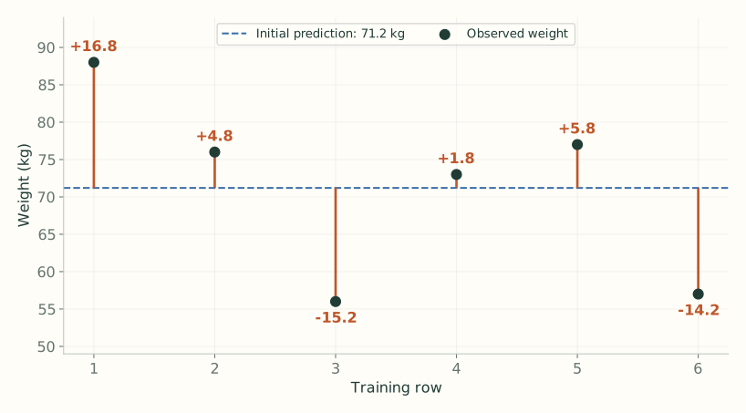
Video 5:50 ↗The lecture predicts weight from height, favorite color, and gender. Before using any feature, predict the average training weight for everybody: about 71.2 kg.
| Row | Height (m) | Color | Gender | Weight (kg) | Residual |
|---|---|---|---|---|---|
| 1 | 1.6 | Blue | Male | 88 | +16.8 |
| 2 | 1.6 | Green | Female | 76 | +4.8 |
| 3 | 1.5 | Blue | Female | 56 | −15.2 |
| 4 | 1.8 | Red | Male | 73 | +1.8 |
| 5 | 1.5 | Green | Male | 77 | +5.8 |
| 6 | 1.4 | Blue | Female | 57 | −14.2 |
The six weights add to 427 kg, so the exact mean is $427/6=71.1666\ldots$. We use 71.2 below to follow the video. This first prediction is deliberately simple: it gives us a starting point whose mistakes we can measure.
It is already a model, just one that ignores the features. Someone short and someone tall both get 71.2. The first tree’s job is to explain which people should move above or below that common starting value.
2. Why predict the residual?
Video 7:17 ↗Row 1 weighs 88 kg, but the model predicts 71.2. The missing amount is $88-71.2=16.8$. Train the new tree to predict that missing amount from the features.
The tree’s output is added to the prediction we already have.
Current prediction + predicted residual = updated prediction.
That is why the tree must predict the remaining error ($+16.8$) rather than the person’s full actual weight ($88$). Because Gradient Boosting adds each tree’s output to the current prediction ($71.2$), if the tree predicted the full weight $88$ instead of the residual $16.8$, adding them together would give $71.2 + 88 = 159.2\text{ kg}$—overshooting the true weight of $88\text{ kg}$ by $71.2\text{ kg}$.
We know actual weights during training, so we can calculate those errors. For a new person we cannot calculate the true error; the tree estimates a correction from their height, color, and gender.
Training on the gaps also keeps the ensemble’s work cumulative. Once earlier trees have explained part of the data, later trees concentrate on the part left unexplained. Training every new tree on the original weights and adding its prediction would repeatedly count the same signal.
3. Fit a small tree to those residuals
Video 7:35 ↗The inputs stay the same. The training target changes from weight to residual. Feature rules group rows with similar residuals into leaves. If several rows share a leaf, the tree uses their mean residual as its output.
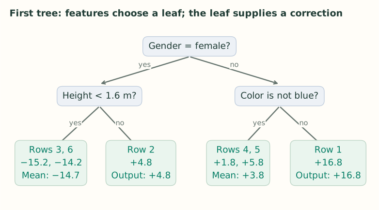
Rows 3 and 6 share a leaf, so its output is $(-15.2-14.2)/2=-14.7$. Their individual errors differ, but both need roughly the same downward correction. A region is simply the group of inputs that follows the rules into one leaf.
Walk through one region
In the pictured tree, a female row follows the left branch. If her height is below 1.6 m, she reaches the leaf containing rows 3 and 6. The complete rule for that region is therefore “female and height below 1.6 m.” Its training rows need corrections of −15.2 and −14.2, so −14.7 is a reasonable shared correction.
For a new person, those feature rules are enough to reach the region. We do not check whether her residual is close to −14.7; her true residual is unknown. The association between that feature region and that correction was learned during training.
Why use one value for both training rows? That is what a tree leaf can represent: one constant output for all inputs reaching it. To give the rows different values, the tree would need another split that separates their features. Small trees deliberately limit that flexibility.
4. Add only part of the correction
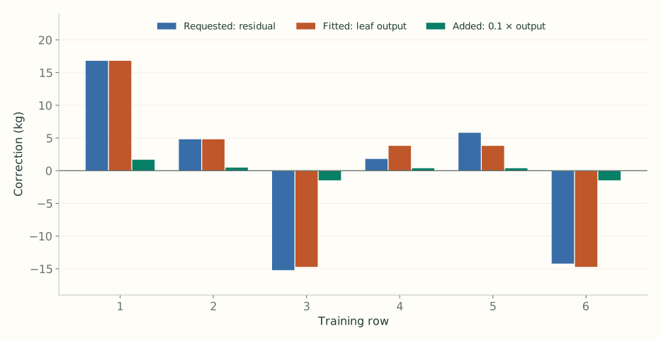
Video 9:11 ↗The lecture scales each tree by a learning rate of 0.1. For row 1:
It is closer to 88, but it has not tried to fix the whole error at once. Small updates let many trees build the fit gradually and can reduce overfitting. A perfect match to a training row alone tells us little about a new person.
The learning rate scales the tree’s contribution; it does not change the actual target, 88.
| Row | Leaf output | Amount added | New prediction | Remaining residual |
|---|---|---|---|---|
| 1 | +16.8 | +1.68 | 72.88 | +15.12 |
| 2 | +4.8 | +0.48 | 71.68 | +4.32 |
| 3 | -14.7 | -1.47 | 69.73 | -13.73 |
| 4 | +3.8 | +0.38 | 71.58 | +1.42 |
| 5 | +3.8 | +0.38 | 71.58 | +5.42 |
| 6 | -14.7 | -1.47 | 69.73 | -12.73 |
Rows 4 and 5 both receive $0.1(3.8)=0.38$, because they share a leaf. Their new predictions are equal, but their new residuals are not: the actual weights remain 73 and 77. The next tree sees those different remaining errors.
The tree’s full fitted correction for rows 3 and 6 would predict 56.5 for both. That lies between their actual weights, 56 and 57. Shrinking the contribution to one tenth moves both predictions only to 69.73 in this round. There is still work for later trees.
5. Predict for a new person
Video 13:50 ↗Start at the initial prediction $F_0$. Send the new person’s features through each trained tree, take the leaf output $h_m(x)$ reached in each, multiply it by the learning rate $\nu$, and add everything:
Here $h_m(x)$ is tree $m$’s correction and $\nu$ is the learning rate. No actual weight or residual is needed to route the new person through a tree.
Training and prediction use different information
| During training | For a new person |
|---|---|
| Use features and actual weights. | Use only the person’s features. |
| Calculate residuals from the current ensemble. | No residual is calculated. |
| Choose feature splits and fit leaf corrections. | Follow the saved feature splits. |
| Append the newly fitted tree to the model. | Add the saved contribution from every tree. |
Adding more trees gives the model more opportunities to learn useful corrections, but also more opportunities to fit noise. Choose the number of rounds using held-out data. A smaller training residual alone does not establish a better prediction for new people.