Machine Learning · Boosting · Gradient Boosting

3. Classification: Main Ideas

September 2026 · Lecture 3 / 4 · 4 min read

Notes on StatQuest with Josh Starmer · Gradient Boost Part 3 · 17:03 video. Explanations and redrawn figures follow the lecture’s worked example.

The additive-tree idea stays the same for binary classification. What changes is the scale: trees add to an unconstrained log-odds score $F \in (-\infty,\infty)$, which the sigmoid converts into a valid probability $p \in (0,1)$.

1. Start with the overall class proportion

Video 0:52 ↗

The six training rows from Lecture 3. Yes = 1 and no = 0.
Row	Likes popcorn	Age	Color	Loves Troll 2 ($y$)
1	Yes	12	Blue	1
2	Yes	87	Green	1
3	No	44	Blue	0
4	Yes	19	Red	0
5	No	32	Green	1
6	No	14	Blue	1

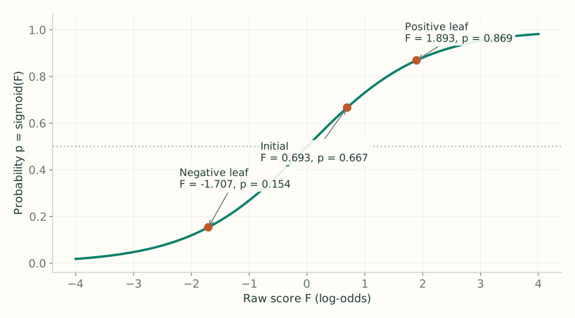
Four of six people love the movie. The initial probability is $p_0=4/6=2/3$. Convert it into the log-odds score stored by the model:

$$F_0=\log\frac{p_0}{1-p_0}=\log\frac{4}{2}=\log 2\approx0.6931.$$

To turn any score $F$ back into a probability, use the sigmoid:

$$p=\frac{e^F}{1+e^F}=\frac1{1+e^{-F}}.$$

At a 0.5 probability threshold, this initial model predicts “yes” for everyone. It has not used anyone’s features yet.

The video often rounds both the score and probability to 0.7. Here we retain $F_0=\log 2$ and $p_0=2/3$, so the two scales stay distinct. This produces slightly different displayed leaf values.

The sigmoid converts initial score 0.693 to probability 0.667. Negative leaf corrections lower the probability; positive corrections raise it. — Add tree outputs on the horizontal, log-odds scale. Then read the resulting probability on the vertical scale. The plotted updates use learning rate 0.8.

2. Calculate the pseudo-residuals

Video 3:37 ↗

$$r_i=y_i-p_i.$$

A “yes” row has residual $1-2/3=1/3$: increase its predicted probability. A “no” row has residual $0-2/3=-2/3$: decrease it. These numbers measure what the current model still gets wrong.

Fit a regression tree using popcorn preference, age, and color to predict these numeric residuals. The final task is classification, but this tree learns numeric corrections.

3. Calculate corrections on the log-odds scale

Video 5:49 ↗

In regression, both the model prediction and the residuals are in the same units (e.g., weight in kg), so a leaf with multiple rows simply outputs their average residual. In classification, however, the ensemble prediction $F$ is a log-odds score while the residuals $r_i = y_i - p_i$ are on the probability scale — so we cannot add raw residuals (or their plain average) directly to $F$.

To convert a leaf $R$’s probability residuals into a log-odds update $\gamma_R$, divide the sum of the residuals in that leaf by the sum of $p_i(1-p_i)$ across the same rows:

$$\gamma_R=\frac{\sum_{i:x_i\in R}(y_i-p_i)}{\sum_{i:x_i\in R}p_i(1-p_i)}.$$

Here the numerator accumulates the net probability error in leaf $R$, and each denominator term $p_i(1-p_i)$ is the local slope (curvature) of the sigmoid that translates a probability gap into a log-odds step (derived via a second-order Taylor expansion in Lecture 4).

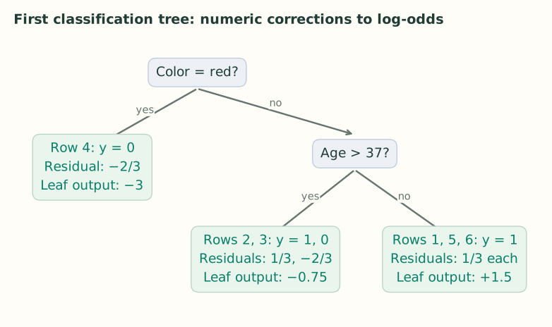
Color red routes row 4 to correction −3. Other colors split at age greater than 37, giving −0.75 for rows 2 and 3 and +1.5 for rows 1, 5 and 6. — The lecture’s first tree, recalculated with exact initial probability 2/3. Leaf outputs are log-odds corrections, not probabilities.

On the first tree, every row starts at the same probability $p_i = 2/3$, so every row contributes $p_i(1-p_i) = (2/3)(1/3) = 2/9$ to its leaf’s denominator (on later trees, each row has its own updated $p_i$, so $p_i(1-p_i)$ must be evaluated per row before summing):

Use one denominator term per training row in the leaf.
Leaf	Residual sum $\sum(y_i-p_i)$	Denominator sum $\sum p_i(1-p_i)$	Plugging into $\gamma_R=\dfrac{\sum(y_i-p_i)}{\sum p_i(1-p_i)}$	Output $\gamma_R$
Red: row 4	$-2/3$	$\tfrac{2}{3}(1-\tfrac{2}{3})=2/9$	$\gamma_R=\dfrac{-2/3}{2/9}$	$-3$
Not red, age > 37: rows 2, 3	$1/3-2/3=-1/3$	$2/9+2/9=4/9$	$\gamma_R=\dfrac{1/3-2/3}{2/9+2/9}=\dfrac{-1/3}{4/9}$	$-0.75$
Not red, age ≤ 37: rows 1, 5, 6	$1/3+1/3+1/3=1$	$2/9+2/9+2/9=6/9$	$\gamma_R=\dfrac{1/3+1/3+1/3}{2/9+2/9+2/9}=\dfrac{1}{6/9}$	$+1.5$

Leaf 1 (Red — row 4): Only row 4 ($y_4=0$, residual $-2/3$) lands here, so there is a single residual in the numerator and a single $2/9$ term in the denominator: $(-2/3) \div (2/9) = -3$.
Leaf 2 (Not red, age > 37 — rows 2 and 3): Row 2 ($y_2=1$, residual $+1/3$) and row 3 ($y_3=0$, residual $-2/3$) share this leaf. Their residuals partially cancel in the numerator ($1/3 - 2/3 = -1/3$), while the denominator sums $p_i(1-p_i)$ for both rows ($2/9 + 2/9 = 4/9$), giving $(-1/3) \div (4/9) = -0.75$.
Leaf 3 (Not red, age ≤ 37 — rows 1, 5, and 6): All three rows have $y_i=1$ (residual $+1/3$ each), so the numerator sums to $3 \times (1/3) = 1$ and the denominator sums three $2/9$ terms to $6/9$, giving $1 \div (6/9) = +1.5$.

4. Add to the score, then convert to probability

Video 8:58 ↗

The lecture uses a large learning rate, 0.8, to make changes easy to see. For row 1, the tree outputs 1.5:

$$F_1(x_1)=\log 2+0.8(1.5)\approx1.8931,$$

$$p_1(x_1)=\operatorname{sigmoid}(1.8931\ldots)\approx0.8691.$$

The probability has moved from 0.6667 toward the observed label 1. Apply the same procedure to the other leaves:

First-round results with exact initialization; values displayed to four decimals.
Rows	Updated score	Updated probability	New residual $y-p$
1, 5, 6	1.8931	0.8691	+0.1309
2	0.0931	0.5233	+0.4767
3	0.0931	0.5233	−0.5233
4	−1.7069	0.1536	−0.1536

Rows 2 and 3 share a leaf but have opposite labels. The shared downward correction helps row 3 and hurts row 2. A single tree need not improve every row; the next tree learns from the errors that remain.

5. Classify a new person

Video 14:28 ↗

Start at the initial log-odds score $F_0$. Route the new person’s features through every trained tree, multiply each reached leaf output $h_m(x)$ by the learning rate $\nu$, and add everything to obtain the final log-odds score $F_M(x)$:

$$F_M(x)=F_0+\nu h_1(x)+\nu h_2(x)+\cdots+\nu h_M(x),\qquad p(x)=\frac{1}{1+e^{-F_M(x)}}.$$

Apply sigmoid once to $F_M(x)$ to get the predicted probability $p(x)$, then compare $p(x)$ against your chosen classification threshold.

Features → one leaf per tree → add log-odds corrections → sigmoid → class.

The leaf values are neither class votes nor probabilities.