Initialization: Break Symmetry and Keep Signals Alive

September 2026 · 4 min read

See why identical hidden units stay identical, derive the per-layer signal multiplier, and track how weight scale compounds across depth.

Weight initialization has two jobs before the first gradient step: ensure hidden units learn distinct features, and keep forward activations and backward gradients from vanishing or exploding as they pass through many layers.

1. Why identical hidden units stay identical

If hidden neurons in a layer start with identical parameters, they compute the same forward activation and receive the same backward gradient on every step. Compare three ways of initializing a layer’s weights $W$ and biases $b$:

• Equal nonzero weights: Every hidden unit computes the exact same activation $\phi(w^\top x+b)$ and receives the exact same gradient during backpropagation. Every deterministic update changes all units identically, so the layer collapses to a single duplicated feature forever.
• All-zero weights ($W=0$): Every hidden unit outputs the same constant activation $\phi(b)$, and incoming-weight gradients vanish on the first step wherever downstream weights are zero, keeping hidden units locked in symmetry.
• Zero biases ($b=0$) with random weights: Sampling distinct random weight rows $w_i\ne w_j$ immediately gives each hidden unit a different preactivation $w_i^\top x$ and a different gradient on the very first pass, so initializing biases to zero is completely safe.

2. How one layer changes signal scale

Scroll the figure horizontally on small screens.

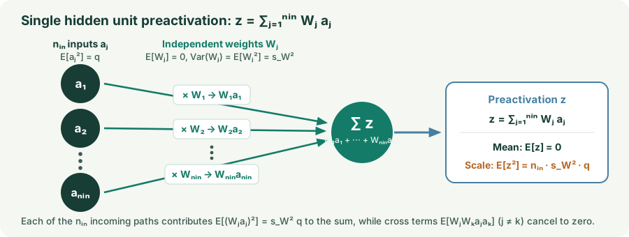
Breaking symmetry only requires random weights, but picking an arbitrary scale like $W_{ij}\sim\mathcal N(0,0.01^2)$ fails in deep networks. Consider a single preactivation $z=\sum_{j=1}^{n_{\rm in}}W_ja_j$, where weights $W_j$ are independent with mean $\mathbb E[W_j]=0$ and variance $\operatorname{Var}(W_j)=\mathbb E[W_j^2]=s_W^2$, and are independent of the inputs $a_j$, which have second moment $q=\mathbb E[a_j^2]$.

First, compute the expected value (mean) $\mathbb E[z]$. By linearity of expectation and the independence of $W_j$ and $a_j$, the mean of $z$ is always zero—even if the inputs $a_j$ have a nonzero mean:

Because $\mathbb E[z]=0$, the output variance equals the output second moment: $\operatorname{Var}(z)=\mathbb E[z^2]-(\mathbb E[z])^2=\mathbb E[z^2]$. Now compute $\mathbb E[z^2]$:

• 1. Expand the square of the sum: Write the square as a product of two sums with indices $j$ and $k$, then split the $n_{\rm in}^2$ pairs into $j=k$ and $j\ne k$:
  $$z^2=\left(\sum_{j=1}^{n_{\rm in}}W_ja_j\right)\left(\sum_{k=1}^{n_{\rm in}}W_ka_k\right)=\sum_{j=1}^{n_{\rm in}}\sum_{k=1}^{n_{\rm in}}W_jW_ka_ja_k=\underbrace{\sum_{j=1}^{n_{\rm in}}W_j^2a_j^2}_{\text{diagonal }(j=k)}+\underbrace{\sum_{j\ne k}W_jW_ka_ja_k}_{\text{cross terms }(j\ne k)}.$$
• 2. Take expectations ($\mathbb E[z^2]$): For $j\ne k$, independence and $\mathbb E[W_j]=0$ make every cross term vanish, while each of the $n_{\rm in}$ diagonal terms contributes $\mathbb E[W_j^2]\mathbb E[a_j^2]=s_W^2q$:
  $$\mathbb E[z^2]=\sum_{j=1}^{n_{\rm in}}\mathbb E[W_j^2]\,\mathbb E[a_j^2]+\sum_{j\ne k}\underbrace{\mathbb E[W_j]}_{0}\underbrace{\mathbb E[W_k]}_{0}\mathbb E[a_ja_k]=n_{\rm in}\,s_W^2\,q,\qquad\operatorname{Var}(z)=\mathbb E[z^2]-\bigl(\mathbb E[z]\bigr)^2=n_{\rm in}\,s_W^2\,q.$$

How variance controls forward signal scale: Because $\mathbb E[z]=0$, the mean tells us nothing about how large the numbers $z$ actually are—positive and negative preactivations cancel out whether $z\in[-10^{-4},10^{-4}]$ or $z\in[-10^4,10^4]$. The typical magnitude (root-mean-square scale) of $z$ is governed by the standard deviation $\sqrt{\operatorname{Var}(z)}=\sqrt{\mathbb E[z^2]}=\bigl(\sqrt{n_{\rm in}}\,s_W\bigr)\sqrt{q}$:

• High variance ($n_{\rm in}s_W^2\gg 1$): Preactivation magnitudes $|z|\sim\sqrt{\operatorname{Var}(z)}$ blow up across the layer. For unbounded activations ($\text{Linear}$, $\text{ReLU}$), feature magnitudes surge and amplify downstream parameter gradients $\partial\ell/\partial W_{l+1}=\delta_{l+1}h_l^\top$; for bounded activations ($\tanh$, $\sigma$), large $|z|$ slams units into their flat saturation tails ($\tanh(z)\approx\pm 1$, $\sigma(z)\approx 0\text{ or }1$) where differences between inputs are wiped out and $\phi'(z)\to 0$.
• Low variance ($n_{\rm in}s_W^2\ll 1$): Preactivations collapse toward $z\approx 0$, shrinking activation magnitudes $|h_l|$ so downstream layers receive almost no signal energy (or a flat constant $\sigma(0)=0.5$ in sigmoid) and weight gradients $\delta_{l+1}h_l^\top$ vanish.
• Scale-preserving variance ($n_{\rm in}s_W^2=1$, i.e. $s_W=1/\sqrt{n_{\rm in}}$): Keeps the output RMS scale $\sqrt{\operatorname{Var}(z)}=\sqrt{q}$ matched to the input scale inside the active region of $\phi(z)$.

Why the recurrence tracks the second moment $\mathbb E[a_j^2]$ instead of variance $\operatorname{Var}(a_j)$: By definition, variance measures expected squared deviation around the mean $\mu_a=\mathbb E[a_j]$, whereas the second moment measures expected squared magnitude around zero. Expanding $\operatorname{Var}(a_j)=\mathbb E[(a_j-\mu_a)^2]$ connects the two:

The second moment and variance coincide only when the inputs are zero-centered ($\mathbb E[a_j]=0$, as in linear layers or odd functions like $\tanh$). For non-negative activations, $\mathbb E[a_j]>0$ and the squared mean $(\mathbb E[a_j])^2$ inflates the next layer’s preactivation variance: sigmoid ($\sigma(z)\in(0,1)$) has mean $\mathbb E[a_j]=0.5$ on symmetric inputs—adding a baseline $(\mathbb E[a_j])^2=0.25$ even when signal spread $\operatorname{Var}(a_j)$ is tiny—and ReLU ($\max(0,z)\ge 0$) has $\mathbb E[a_j]>0$.

3. Compounding across depth: forward and backward

Now stack $L$ linear layers in a chain: $h_l=W_lh_{l-1}$ for $l=1,2,\dots,L$, starting from input $h_0=x$ with coordinate second moment $q_0=\mathbb E[h_{0,j}^2]$. Suppose every layer has width $n$ ($n_{\rm in}=n$) and each weight matrix $W_l\in\mathbb R^{n\times n}$ has independent zero-mean entries of variance $s_W^2$, independent of the incoming activations $h_{l-1}$.

Let $q_l=\mathbb E[h_{l,i}^2]$ denote the second moment of a coordinate after layer $l$. Applying our single-layer result from Section 2 to layer $l$—where $h_{l,i}=\sum_{j=1}^n W_{l,ij}h_{l-1,j}$ sums $n$ inputs of second moment $q_{l-1}$—shows that each layer multiplies the signal’s second moment by the per-layer factor $c=ns_W^2$. Unrolling that recurrence from layer $1$ through layer $L$ multiplies by $c$ at every step:

Because depth $L$ sits in the exponent, the signal scale forms a geometric progression with ratio $c=ns_W^2$, splitting initialization into three regimes:

• Vanishing forward signal ($c<1$, or $s_W<1/\sqrt{n_{\rm in}}$): $c^L\to 0$ exponentially with depth $L$, shrinking activations toward zero before they reach the output.
• Exploding forward signal ($c>1$, or $s_W>1/\sqrt{n_{\rm in}}$): $c^L\to\infty$ exponentially with depth $L$, causing activations to blow up across deep stacks.
• Scale-preserving boundary ($c=1$, or $s_W=1/\sqrt{n_{\rm in}}$): $1^L=1$ for every $L$, keeping $q_L=q_0$ constant no matter how deep the network is. Setting the per-layer forward multiplier equal to $1$ gives the forward weight-variance condition:
  $$\begin{aligned}n_{\rm in}\cdot\operatorname{Var}(W)&=1\\\operatorname{Var}(W)=s_W^2&=\frac{1}{n_{\rm in}}\\\sqrt{\operatorname{Var}(W)}=s_W&=\sqrt{\frac{1}{n_{\rm in}}}=\frac{1}{\sqrt{n_{\rm in}}}.\end{aligned}$$

Backward pass: why $n_{\rm out}$ appears by the exact same derivation

To keep layer numbers and neuron numbers completely distinct, write the layer index in the superscript—with left layer $(l)$ containing $n_{\rm in}$ neurons (indexed by $j=1,\dots,n_{\rm in}$) and right layer $(l+1)$ containing $n_{\rm out}$ neurons (indexed by $i=1,\dots,n_{\rm out}$). The weight matrix sitting between them belongs to the right layer, $W^{(l+1)}\in\mathbb R^{n_{\rm out}\times n_{\rm in}}$, where $i$ picks the neuron in the right layer $(l+1)$ and $j$ picks the neuron in the left layer $(l)$:

• Forward pass (left layer $l\to$ right layer $l+1$, $z^{(l+1)}=W^{(l+1)}a^{(l)}$): One neuron $z_i^{(l+1)}$ in the right layer sums over all $n_{\rm in}$ neurons $j=1,\dots,n_{\rm in}$ from the left layer:
  $$z_i^{(l+1)}=\sum_{j=1}^{n_{\rm in}}W_{i,j}^{(l+1)}a_j^{(l)}.$$
• Backward pass (right layer $l+1\to$ left layer $l$, $\delta^{(l)}=(W^{(l+1)})^\top\delta^{(l+1)}$): Because neuron $a_j^{(l)}$ in the left layer sent its signal to all $n_{\rm out}$ neurons $z_1^{(l+1)},\dots,z_{n_{\rm out}}^{(l+1)}$ in the right layer via the right layer’s weights $W_{i,j}^{(l+1)}$, the chain rule says its gradient $\delta_j^{(l)}=\frac{\partial\ell}{\partial a_j^{(l)}}$ must sum the upstream gradients $\delta_i^{(l+1)}=\frac{\partial\ell}{\partial z_i^{(l+1)}}$ returning from all $n_{\rm out}$ neurons of the right layer $(l+1)$:
  $$\delta_j^{(l)}=\frac{\partial\ell}{\partial a_j^{(l)}}=\sum_{i=1}^{n_{\rm out}}\underbrace{\frac{\partial\ell}{\partial z_i^{(l+1)}}}_{\delta_i^{(l+1)}}\underbrace{\frac{\partial z_i^{(l+1)}}{\partial a_j^{(l)}}}_{W_{i,j}^{(l+1)}}=\sum_{i=1}^{n_{\rm out}}W_{i,j}^{(l+1)}\delta_i^{(l+1)}.$$

Notice that $\delta_j^{(l)}=\sum_{i=1}^{n_{\rm out}}W_{i,j}^{(l+1)}\delta_i^{(l+1)}$ has the exact same mathematical structure as $z_i^{(l+1)}=\sum_{j=1}^{n_{\rm in}}W_{i,j}^{(l+1)}a_j^{(l)}$—using the right layer’s weights $W^{(l+1)}$, with the sum running over the $n_{\rm out}$ neurons $i=1,\dots,n_{\rm out}$ of the right layer instead of the $n_{\rm in}$ neurons $j=1,\dots,n_{\rm in}$ of the left layer. Letting $\tilde q_{l+1}=\mathbb E[(\delta_i^{(l+1)})^2]$ be the gradient second moment at the right layer $(l+1)$, with $\mathbb E[W_{i,j}^{(l+1)}]=0$ and $\operatorname{Var}(W_{i,j}^{(l+1)})=\mathbb E[(W_{i,j}^{(l+1)})^2]=s_W^2$ independent of $\delta_i^{(l+1)}$, we follow the exact same three steps:

• 1. Mean is zero ($\mathbb E[\delta_j^{(l)}]=0$):
  $$\mathbb E\bigl[\delta_j^{(l)}\bigr]=\mathbb E\!\left[\sum_{i=1}^{n_{\rm out}}W_{i,j}^{(l+1)}\delta_i^{(l+1)}\right]=\sum_{i=1}^{n_{\rm out}}\underbrace{\mathbb E\bigl[W_{i,j}^{(l+1)}\bigr]}_{0}\mathbb E\bigl[\delta_i^{(l+1)}\bigr]=0.$$
• 2. Expand the square of the sum into diagonal ($i=k$) and cross ($i\ne k$) terms:
  $$\bigl(\delta_j^{(l)}\bigr)^2=\left(\sum_{i=1}^{n_{\rm out}}W_{i,j}^{(l+1)}\delta_i^{(l+1)}\right)\left(\sum_{k=1}^{n_{\rm out}}W_{k,j}^{(l+1)}\delta_k^{(l+1)}\right)=\underbrace{\sum_{i=1}^{n_{\rm out}}\bigl(W_{i,j}^{(l+1)}\bigr)^2\bigl(\delta_i^{(l+1)}\bigr)^2}_{\text{diagonal }(i=k)}+\underbrace{\sum_{i\ne k}W_{i,j}^{(l+1)}W_{k,j}^{(l+1)}\delta_i^{(l+1)}\delta_k^{(l+1)}}_{\text{cross terms }(i\ne k)}.$$
• 3. Take expectations ($\tilde q_l=\mathbb E[(\delta_j^{(l)})^2]$): Every $i\ne k$ cross term drops out because $\mathbb E[W_{i,j}^{(l+1)}]=0$, leaving $n_{\rm out}$ diagonal terms each equal to $s_W^2\tilde q_{l+1}$:
  $$\operatorname{Var}\bigl(\delta_j^{(l)}\bigr)=\tilde q_l=\mathbb E\bigl[(\delta_j^{(l)})^2\bigr]=\sum_{i=1}^{n_{\rm out}}\mathbb E\bigl[(W_{i,j}^{(l+1)})^2\bigr]\,\mathbb E\bigl[(\delta_i^{(l+1)})^2\bigr]+\sum_{i\ne k}\underbrace{\mathbb E\bigl[W_{i,j}^{(l+1)}\bigr]}_{0}\underbrace{\mathbb E\bigl[W_{k,j}^{(l+1)}\bigr]}_{0}\mathbb E\bigl[\delta_i^{(l+1)}\delta_k^{(l+1)}\bigr]=n_{\rm out}\,s_W^2\,\tilde q_{l+1}.$$

Unrolling this backward recurrence $\tilde q_l=(n_{\rm out}\,s_W^2)\,\tilde q_{l+1}$ across $L$ layers from the output gradient $\tilde q_L$ back to the input gradient $\tilde q_0$ gives $\tilde q_0=(n_{\rm out}\,s_W^2)^L\tilde q_L$. Requiring the backward gradient variance to stay constant across layers ($\tilde q_l=\tilde q_{l+1}$) sets the backward multiplier equal to $1$:

• Forward pass: each output neuron in layer $(l+1)$ sums $n_{\rm in}$ incoming connections from layer $(l)$ $\implies$ variance scales by $n_{\rm in}\cdot\operatorname{Var}(W)$ (preserving forward scale requires $\operatorname{Var}(W)=1/n_{\rm in}$, i.e. $s_W=\sqrt{1/n_{\rm in}}$).
• Backward pass: each input neuron in layer $(l)$ sums $n_{\rm out}$ returning gradient connections from layer $(l+1)$ via $W^{(l+1)}$ $\implies$ gradient variance scales by $n_{\rm out}\cdot\operatorname{Var}(W)$ (preserving backward gradient scale requires $\operatorname{Var}(W)=1/n_{\rm out}$, i.e. $s_W=\sqrt{1/n_{\rm out}}$).

Resolving the conflict when $n_{\rm in}\ne n_{\rm out}$

Unless a layer has equal input and output widths ($n_{\rm in}=n_{\rm out}$), the forward and backward conditions give two conflicting equations for the same weight variance $\operatorname{Var}(W)=s_W^2$:

Because a single weight matrix $W^{(l+1)}$ cannot satisfy both at once when $n_{\rm in}\ne n_{\rm out}$, Xavier (Glorot) initialization compromises by averaging the two fan counts $\bigl(n_{\rm avg}=\frac{n_{\rm in}+n_{\rm out}}{2}\bigr)$:

Sources

Glorot and Bengio, Understanding the Difficulty of Training Deep Feedforward Neural Networks; He et al., Delving Deep into Rectifiers; Saxe et al., Deep Linear Network Dynamics.