SGD with Momentum: Remembering a Direction

September 2026 · 6 min read + interactive lab

Unroll the momentum buffer, distinguish velocity from displacement, and see why narrow valleys are difficult.

In a narrow valley, SGD repeatedly crosses the steep direction while inching along the flat direction. Momentum gives the optimizer a memory: gradient components that keep pointing the same way accumulate, while rapidly reversing components partially cancel. That is the mechanism behind the familiar “rolling ball” picture—but the actual recurrence is more useful than the analogy.

1. A buffer is a weighted history

Start with a zero buffer $b_0=0$. The heavy-ball convention used in this chapter is

The gradient $g_t$ is evaluated at the current parameter $w_{t-1}$. The coefficient $\beta$ controls how much of the previous buffer survives. The buffer has gradient units; the displacement $\Delta w_t=-\eta_t b_t$ has parameter units. A positive buffer component moves that parameter in the negative direction.

Substitute the recurrence into itself:

Older gradients receive exponentially smaller weights. They were evaluated at older parameter values, so this history provides persistence at the cost of lag. Momentum can keep moving through a point where the current gradient is zero.

For a constant gradient $g$, the geometric series sums to the steady-state limit:

Consequently, adding momentum while keeping the same learning rate $\eta$ multiplies the sustained step magnitude along a steady direction by $1/(1-\beta)$.

2. Two conventions that look deceptively similar

1. Heavy-ball ($b_t$) vs. EMA ($m_t$): equivalent after rescaling the learning rate. Many papers write momentum as an exponential moving average with $m_0=0$:

Unrolling $m_t$ and comparing with $b_t=\beta b_{t-1}+g_t$ ($b_0=0$) shows that $m_t$ is simply $b_t$ scaled by $(1-\beta)$:

Therefore, the two rules produce the exact same parameter updates if and only if the learning rates are scaled by $1-\beta$:

2. Gradient buffer ($b_t$) vs. velocity buffer ($v_t$): equivalent for fixed $\eta$, different under a schedule $\eta_t$. Another convention puts the learning rate inside the recurrence ($v_0=0$):

Compare the step-2 displacement $\Delta w_2$ under both conventions:

If $\eta_1=\eta_2=\eta$ is constant, both give $v_t=-\eta b_t$ and are identical. When $\eta_t$ changes (such as during warmup or decay), $-\eta_t b_t$ rescales the entire stored history by the new rate $\eta_2$, whereas $v_t$ keeps the old rate $\eta_1$ on past gradients.

3. Momentum changes the dynamics, not the loss

For $L(w)=\tfrac12\lambda w^2$ and constant learning rate, combine the parameter and buffer recurrences to eliminate the buffer:

Unlike SGD, the next position depends on two earlier positions. A suitably chosen pair $(\eta,\beta)$ can make progress in flat directions much faster while controlling sharp-direction oscillations. But old direction information can also cause overshoot and slow the response to a turn. Large momentum is not a guarantee of faster convergence.

For a single positive-curvature quadratic mode, $0\le\beta<1$ and $0<\eta\lambda<2(1+\beta)$ give stable heavy-ball dynamics. Stability only means eventual decay in this idealized setting; the transient can still oscillate substantially. Stochastic gradients and a changing neural-network Hessian complicate this picture.

4. Lab: watch the stored direction

This uses the same eight-example quadratic dataset as the SGD chapter. The default full gradient removes sampling noise so you can first see the effect of curvature. The readout exposes the current buffer and the displacement separately.

• Start without memory: set $\beta=0$, full gradient, $\eta=0.03$, and $\kappa=20$. Inspect progress along the long axis of the contours.
• Add persistence: repeat with $\beta=0.9$. Notice both the increased progress and the overshoot; compare loss over several steps, not just one.
• Add noise: select one sampled row. Near the optimum, the buffer keeps contributions from past noisy batches. More memory does not make those contributions disappear.

5. Where Nesterov momentum differs

The conceptual Nesterov form asks for a gradient at a lookahead point. Using a displacement velocity and a constant rate:

Scroll the figure horizontally on small screens.

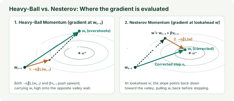
The gradient can correct the direction after accounting for where the stored velocity is about to take us. This is different from simply increasing $\beta$. Libraries may implement an algebraically rearranged form in different parameter coordinates. For example, PyTorch forms a buffer and uses $g_t+\beta b_t$ for its Nesterov update. Do not implement both a lookahead move and that extra term without deriving the intended convention.

The classic Sutskever et al. study discusses momentum and initialization in deep learning. Its results support taking momentum dynamics seriously; they do not turn a particular coefficient into a universal choice.

6. Implementation and state

# Heavy-ball convention used in this chapter.
# b persists across batches and starts at zero.
b = beta * b + grad
parameter -= learning_rate * b

# Corresponding PyTorch configuration:
optimizer = torch.optim.SGD(
    model.parameters(), lr=0.03, momentum=0.9,
    dampening=0, nesterov=False, weight_decay=0
)

Unlike plain SGD (which stores no state between steps), momentum stores one extra number—the buffer value $b_{t,i}$—for every individual model parameter $w_i$. In code, each parameter tensor W of shape $(d_{\text{out}}, d_{\text{in}})$ gets a matching buffer tensor b of the same shape $(d_{\text{out}}, d_{\text{in}})$, doubling the parameter memory footprint compared to stateless SGD ($+4\text{ bytes/parameter}$ in FP32). Because b carries the accumulated direction across steps, always save optimizer.state_dict() alongside model weights when checkpointing.

7. Questions worth answering

Sources

Sutskever et al., On the Importance of Initialization and Momentum in Deep Learning; PyTorch SGD: momentum conventions and Nesterov implementation. The sequence, figures, and quadratic experiments are original teaching examples.