Deep Learning · Data Imbalance in Deep LearningChapter 12 / 12

Post-Hoc Calibration, Cost-Optimal Thresholds, and Label-Shift Correction

October 2026 · 7 min read

Derive the cost-optimal threshold $p^*=C_{\text{FP}}/(C_{\text{FP}}+C_{\text{FN}})$ and the exact Bayes prior-shift formula that recalibrates probabilities after oversampling, undersampling, or class-weighted training.

Suppose your model is already trained. Two critical questions remain at deployment time: (1) What probability threshold $p^*$ should trigger a positive decision when false negatives and false positives have unequal costs? (2) If you trained with oversampling, undersampling, or class weights $\alpha_k$, why are the model’s output probabilities $\hat p$ severely miscalibrated—and how do you recover the true deployment probability $p_{\text{real}}(y=1\mid x)$ in closed form?

1. Derive the Bayes cost-optimal decision threshold $p^*$

Let $p=P(y=1\mid x)$ be the true calibrated probability that input $x$ belongs to the positive class. Suppose a false positive ($\hat y=1$ when $y=0$) incurs cost $C_{\text{FP}}>0$ and a false negative ($\hat y=0$ when $y=1$) incurs cost $C_{\text{FN}}>0$ (with zero cost for correct predictions). Compare the expected cost of predicting $\hat y=1$ versus $\hat y=0$:

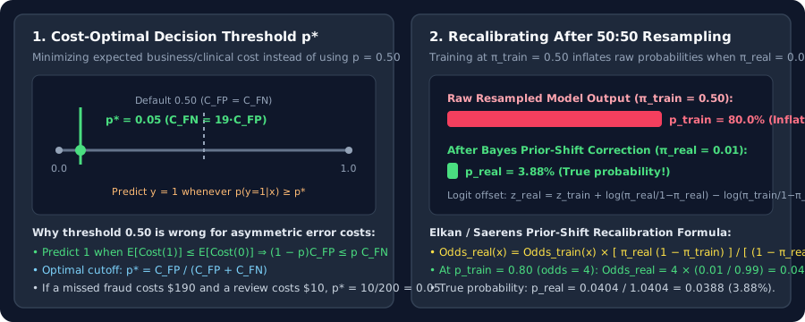
$$\begin{aligned}\mathbb E[\text{Cost}(\hat y=1\mid x)]&=P(y=0\mid x)\,C_{\text{FP}}=(1-p)C_{\text{FP}},\\[4pt]\mathbb E[\text{Cost}(\hat y=0\mid x)]&=P(y=1\mid x)\,C_{\text{FN}}=p\,C_{\text{FN}}.\end{aligned}$$

Predicting $\hat y=1$ is optimal whenever $\mathbb E[\text{Cost}(\hat y=1\mid x)]\le\mathbb E[\text{Cost}(\hat y=0\mid x)]$. Solving for $p$ gives the exact Bayes cost-optimal threshold $p^*$:

$$(1-p)C_{\text{FP}}\le p\,C_{\text{FN}}\implies C_{\text{FP}}\le p(C_{\text{FP}}+C_{\text{FN}})\implies p\ge p^*=\frac{C_{\text{FP}}}{C_{\text{FP}}+C_{\text{FN}}}.$$

Notice why the default $0.50$ threshold is almost never optimal on rare events: $p^*=0.50$ implicitly assumes $C_{\text{FP}}=C_{\text{FN}}$. If missing a fraudulent transaction costs $C_{\text{FN}}=\$190$ while reviewing a flagged transaction costs $C_{\text{FP}}=\$10$, the optimal threshold is $p^*=\frac{10}{10+190}=0.05$ ($5\%$).

Left: cost-optimal threshold p* = 0.05 when C_FN = 19 C_FP compared to default 0.50. Right: Bayes prior-shift recalibration converting an inflated 80% resampled probability back to the true 3.88% deployment probability. — Left: when a missed positive costs $19\times$ more than a false alarm, the optimal cutoff drops from $0.50$ to $p^*=0.05$. Right: a model trained on $50{:}50$ resampled data outputs $p_{\text{train}}=80.0\%$, which corresponds to a true probability of only $p_{\text{real}}=3.88\%$ when $\pi_{\text{real}}=0.01$.

2. Why resampling warps probabilities—and the exact Bayes correction

When you train a model using class-balanced sampling ($\pi_{\text{train}}=0.50$) or positive class weight $\alpha_+$, the model’s output $p_{\text{train}}(y=1\mid x)$ is calibrated for $\pi_{\text{train}}=0.50$, not for the real deployment prevalence $\pi_{\text{real}}=0.01$. Because resampling changes the class prior $P(y)$ while leaving the within-class feature distribution $P(x\mid y)$ unchanged, Bayes’ theorem relates the real posterior odds to the training posterior odds:

$$\begin{aligned}\underbrace{\frac{p_{\text{real}}(y=1\mid x)}{1-p_{\text{real}}(y=1\mid x)}}_{\text{real posterior odds}}&=\frac{P(x\mid y=1)}{P(x\mid y=0)}\cdot\frac{\pi_{\text{real}}}{1-\pi_{\text{real}}}=\underbrace{\frac{p_{\text{train}}(y=1\mid x)}{1-p_{\text{train}}(y=1\mid x)}}_{\text{training posterior odds}}\cdot\underbrace{\frac{\pi_{\text{real}}}{1-\pi_{\text{real}}}\cdot\frac{1-\pi_{\text{train}}}{\pi_{\text{train}}}}_{\text{prior odds ratio }\rho}.\end{aligned}$$

In logit space ($z=\log\frac{p}{1-p}$), multiplying the odds by $\rho$ is simply adding $\log\rho$ to the logit $z_{\text{train}}$:

$$\begin{aligned}z_{\text{real}}(x)&=z_{\text{train}}(x)+\log\frac{\pi_{\text{real}}}{1-\pi_{\text{real}}}-\log\frac{\pi_{\text{train}}}{1-\pi_{\text{train}}},\\[6pt]p_{\text{real}}(y=1\mid x)&=\sigma\bigl(z_{\text{real}}(x)\bigr)=\frac{\rho\,p_{\text{train}}(x)}{\rho\,p_{\text{train}}(x)+1-p_{\text{train}}(x)}.\end{aligned}$$

Worked numerical check: Suppose you balanced a $\pi_{\text{real}}=0.01$ dataset to $\pi_{\text{train}}=0.50$, and on a test customer the balanced model predicts $p_{\text{train}}=0.80$ (training odds $=0.80/0.20=4.0$):

$$\begin{aligned}\rho&=\frac{0.01}{0.99}\cdot\frac{0.50}{0.50}=\frac{1}{99}\approx 0.0101,\\[4pt]\text{Real odds}&=4.0\times\frac{1}{99}=\frac{4}{99}\approx 0.0404\implies p_{\text{real}}=\frac{4/99}{1+4/99}=\frac{4}{103}\approx 0.0388\;(3.88\%!).\end{aligned}$$

Without prior-shift correction, reporting “$80\%$ fraud probability” to a downstream risk engine when the true probability is $3.88\%$ causes catastrophic over-triggering!

3. End-to-end decision guide across all 12 chapters

Problem Regime	Recommended Training Pipeline	Inference / Calibration Rule
Binary tabular / rare event ($\pi_+\le 1\%$)	Initialize bias $b_0=\log(\pi_+/\pi_-)$; train with standard or Focal Loss; tune threshold on validation PR curve.	If undersampled/oversampled, apply prior-shift correction $\rho$, then threshold at $p^*=C_{\text{FP}}/(C_{\text{FP}}+C_{\text{FN}})$.
Multi-class long-tailed vision/audio ($\text{IF}=100\text{–}1000$)	Option A (1-stage): Balanced Softmax / Logit Adjustment ($z_k+\tau\log\pi_k$). Option B (2-stage): Stage 1 at $q=1$, Stage 2 with cRT or $\tau$-norm.	Predict $\arg\max_k z_k$ (for Balanced Softmax / cRT) or $\arg\max_k(z_k-\tau\log\pi_k)$ (post-hoc LA).
Dense segmentation ($99.8\%$ background pixels)	Combo Loss: $0.5\,L_{\text{BCE}}+0.5\,L_{\text{Dice}}$ (or Tversky with $\alpha=0.3,\beta=0.7$ when recall is critical).	Tune foreground mask threshold on validation Dice / IoU.
Multi-label tagging ($K\ge 50$ independent classes)	Asymmetric Loss (ASL) with $\gamma_+=0,\gamma_-=4$, probability shift $m=0.05$.	Per-class threshold tuned for validation Macro-$F_1$.

4. Questions worth answering

If you train with positive class weight $\alpha_+>1$ and negative weight $\alpha_-=1$ in binary cross-entropy, what effective training prior $\pi_{\text{train}}$ does the model’s probability correspond to?

Multiplying positive losses by $\alpha_+$ is equivalent to multiplying the positive count $n_+$ by $\alpha_+$, so the effective training prior odds are $\frac{\pi_{\text{train}}}{1-\pi_{\text{train}}}=\alpha_+\frac{\pi_{\text{real}}}{1-\pi_{\text{real}}}$. Subtracting $\log\alpha_+$ from the trained logit recovers the true calibrated log-odds!

Should you tune the decision threshold $p^*$ on the training set or a held-out validation set?

Always on a held-out validation set whose class distribution matches deployment (or after applying the prior-shift formula). On the training set, neural networks memorize minority examples with $p_i\approx 0.99$, which biases the threshold upward.