Random Undersampling
Random undersampling makes training smaller by selecting fewer rows from the classes you choose to reduce. In the common binary case, keep the minority examples and randomly retain only some majority examples.
This can reduce training work and change the class influence. Its central tradeoff is coverage: a row that is not selected cannot teach this fitted model anything. We will track both the retained identities and a particular majority example that may disappear.
Select a subset, not a new measurement
There are six negatives A–F and two positives G–H. Select two of the six negatives without replacement, so no negative can be selected twice. Keep both positives. The resulting training set has four rows, two from each class.
One draw keeps F and C; another keeps C and B. Both have the same class counts. They contain different evidence.
The majority class can contain rare, useful situations
Now give the rows a one-dimensional feature. A–E have values 0–4, F has value 9, and positives G–H have values 10 and 11. F is the only observed negative close to those positives.
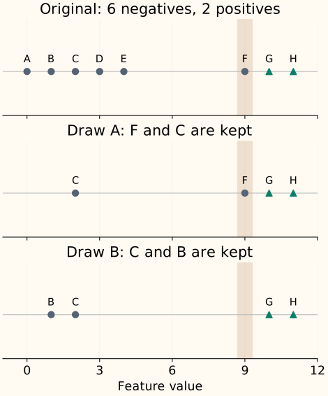
F might represent an unusual operating condition within the majority class. Removing it may weaken coverage even though the majority class still has many examples elsewhere. This figure identifies missing evidence; it does not prove which resulting classifier will perform better.
Keeping two of six negatives gives every particular negative a 2 / 6 = 1/3 chance of retention. F is absent in two thirds of possible uniform draws. Repeating an experiment with a different seed measures sensitivity to this selection; it does not recover F for a model trained on a draw that omitted it.
Probability of losing an entire majority subgroup
Suppose the majority class has $N$ rows, a subgroup occupies $r$ of them, and we retain $m$ rows uniformly without replacement. There are $\binom{N}{m}$ possible retained subsets; $\binom{N-r}{m}$ use only rows outside the subgroup. The symbol $\binom{a}{b}$ counts ways to choose $b$ distinct objects from $a$.
When $m>N-r$, omission is impossible and the numerator is zero. With N = 6, r = 1 and m = 2, the probability is 10 / 15 = 2/3. The formula describes sampling coverage, not the eventual classifier’s error rate.
Because full balancing shrinks every class down to the smallest class’s count, it can discard almost the entire dataset: with 990 negatives and 10 positives, sampling_strategy="auto" keeps only 20 rows in total, whereas retaining 100 negatives keeps 110.
Without replacement means distinct retained rows
RandomUnderSampler defaults to replacement=False, as do this chapter’s examples. A target of two negatives then means two distinct negative source rows. With replacement=True, the selected output can contain duplicate identities, reducing distinct coverage further even if its row count is unchanged.
The algorithm samples by class and does not examine feature distances to decide which majority rows are useful. Methods that select rows based on boundaries or clusters make additional assumptions; they are different algorithms. When minority coverage itself is the limiting factor, neither copying positives nor dropping negatives creates new positive situations—the next chapter introduces SMOTE’s interpolation assumption and shows how to inspect the feature vectors it generates.
References and further reading
- Imbalanced-learn: RandomUnderSampler — final class counts, replacement options and retained source indices.
- Imbalanced-learn: random undersampling — class-wise random selection and its distinction from more structured selection methods.