Deep Learning · Data Imbalance in Deep Learning · Class Imbalance and Resampling

Evaluating Under Imbalance

September 2026 · 16 min read

Start with the operating decision

A score becomes a positive prediction when it passes a chosen threshold. For the earlier detector on $1{,}000$ items, the four outcomes are $\text{TP} = 8$ (predicted positive and actually positive), $\text{FP} = 20$ (predicted positive, actually negative—false alarms), $\text{FN} = 2$ (predicted negative, actually positive—missed defects), and $\text{TN} = 970$ (predicted negative and actually negative). Before reading the table, notice what each denominator sum represents:

$\text{TP} + \text{FP} = 8 + 20 = 28$ $\to$ Total positives predicted (all alerts): dividing $\text{TP}$ by $\text{TP}+\text{FP}$ (Precision) asks: out of all positives predicted, how many were actually positive?
$\text{TP} + \text{FN} = 8 + 2 = 10$ $\to$ Total actual positives in the data: dividing $\text{TP}$ by $\text{TP}+\text{FN}$ (Recall) asks: out of all actual positives in the data, how many did we catch?
$\text{TN} + \text{FP} = 970 + 20 = 990$ $\to$ Total actual negatives in the data: dividing $\text{TN}$ by $\text{TN}+\text{FP}$ (specificity / negative recall) asks: out of all actual negatives in the data, how many were kept negative?
$\text{TP} + \text{FP} + \text{FN} + \text{TN} = 1{,}000$ $\to$ Total items in the data.

Metric	Formula	Calculation here	What it emphasizes
Precision	$\dfrac{\text{TP}}{\text{TP}+\text{FP}}$	$8 / (8 + 20) = 8 / 28 \approx 28.6\%$	The fraction of alerts that are real positives.
Recall	$\dfrac{\text{TP}}{\text{TP}+\text{FN}}$	$8 / (8 + 2) = 8 / 10 = 80\%$	The fraction of actual positives that are detected.
F1	$\dfrac{2\cdot\text{Prec}\cdot\text{Rec}}{\text{Prec}+\text{Rec}}$	$2 \times 8 / (2 \times 8 + 20 + 2) \approx 0.4211$	A harmonic-mean summary of precision and recall; it does not include TN.
Balanced accuracy	$\dfrac{1}{2}\!\left(\dfrac{\text{TP}}{\text{TP}+\text{FN}} + \dfrac{\text{TN}}{\text{TN}+\text{FP}}\right)$	$(8 / 10 + 970 / 990) / 2 \approx 89.0\%$	Equal weight for each class’s recall, regardless of its count.
Alert load	$\dfrac{\text{TP}+\text{FP}}{\text{TP}+\text{FP}+\text{FN}+\text{TN}}$	$(8 + 20) / 1{,}000 = 28 / 1{,}000 = 2.8\%$	The fraction of incoming cases sent to the positive action.

Balanced accuracy averages positive recall with negative recall, also called specificity. F1 summarizes a different tradeoff. Neither automatically represents the costs of mistakes or a fixed review capacity. If reviewers can inspect only 20 cases per day, report performance at that capacity and state how tied scores are handled.

Precision changes when positives become rarer

Keep a detector’s recall at 80% and its false positive rate at 2%. The latter means it flags 2% of actual negatives, not that 2% of its alerts are wrong. Apply those rates to 10,000 cases with 1% positive prevalence:

There are 100 positives, of which 80 are detected, and 9,900 negatives, of which 198 raise false alarms. Precision is 80 / (80 + 198) ≈ 28.8%. A small false positive rate can create many false alerts because it acts on a large negative population.

Same recall and false positive rate, different population

ACTUAL POSITIVES100 cases80 detected; 20 missed

ACTUAL NEGATIVES9,900 cases198 false alarms; 9,702 correct negatives

Alerts: 80 true positives (blue) + 198 false positives (orange).

Precision: 28.8%. Recall stays 80%; false positive rate stays 2%.

The bar shows the composition of alerts, not the whole dataset. This controlled calculation holds both class-conditional error rates fixed; a real population shift can change those rates too.

The short formula behind the population calculation

Write $\pi$ for the positive fraction, TPR for recall and FPR for the false positive rate. The true-positive fraction of all cases is TPR × $\pi$; the false-positive fraction is FPR × $(1-\pi)$. Dividing the first by their sum gives

$$\text{precision}=\frac{\operatorname{TPR}\,\pi}{\operatorname{TPR}\,\pi+\operatorname{FPR}(1-\pi)}.$$

This is why precision from a deliberately balanced evaluation set does not directly predict alert quality in a much rarer-positive population.

ROC and precision–recall curves: why ROC-AUC looks overly optimistic under class imbalance

Sweeping a threshold produces many confusion matrices. A ROC curve plots $\operatorname{TPR}=\frac{\text{TP}}{\text{TP}+\text{FN}}$ (Recall) against $\operatorname{FPR}=\frac{\text{FP}}{\text{FP}+\text{TN}}$. A precision–recall (PR) curve plots $\operatorname{Precision}=\frac{\text{TP}}{\text{TP}+\text{FP}}$ against $\operatorname{Recall}=\frac{\text{TP}}{\text{TP}+\text{FN}}$.

Why ROC-AUC can be misleading under severe class imbalance while PR-AUC exposes false alarms: Notice the denominators of the two curves on a $1{:}99$ imbalanced dataset with $n_+=10$ actual positives and $n_-=990$ actual negatives, where a threshold catches $9$ positives ($\text{TP}=9,\text{FN}=1$) and triggers $90$ false alarms ($\text{FP}=90,\text{TN}=900$):

$$\begin{aligned}\textbf{ROC curve axes:}\quad \operatorname{TPR}&=\frac{\text{TP}}{\text{TP}+\text{FN}}=\frac{9}{10}=90.0\%,\qquad \operatorname{FPR}=\frac{\text{FP}}{\text{FP}+\text{TN}}=\frac{90}{990}=9.1\%,\\[6pt]\textbf{PR curve axes:}\quad \operatorname{Recall}&=\frac{\text{TP}}{\text{TP}+\text{FN}}=\frac{9}{10}=90.0\%,\qquad \operatorname{Precision}=\frac{\text{TP}}{\text{TP}+\text{FP}}=\frac{9}{9+90}=\frac{9}{99}=9.1\%.\end{aligned}$$

Why ROC and ROC-AUC stay deceptively high: $\operatorname{TPR}=\text{TP}/n_+$ is normalized purely within actual positives and $\operatorname{FPR}=\text{FP}/n_-$ is normalized purely within actual negatives—neither axis ever mixes $n_+$ and $n_-$. Dividing $90$ false alarms by all $990$ negatives gives a tiny $\operatorname{FPR}=9.1\%$, placing $(0.091, 0.900)$ near the top-left corner ($\operatorname{ROC-AUC}\approx 0.95$).
Why Precision and PR-AUC collapse: $\operatorname{Precision}=\frac{\text{TP}}{\text{TP}+\text{FP}}$ puts true detections ($\text{TP}=9$) and false alarms ($\text{FP}=90$) in the same denominator ($\text{TP}+\text{FP}=99$), immediately revealing that $10$ out of every $11$ positive alerts are false alarms ($\operatorname{Precision}=9.1\%$). Dividing top and bottom by total items shows that the imbalance ratio $\frac{1-\pi}{\pi}=\frac{n_-}{n_+}$ directly multiplies $\operatorname{FPR}$ in the denominator of Precision:

$$\operatorname{Precision}=\frac{\text{TP}}{\text{TP}+\text{FP}}=\frac{\pi\,\operatorname{TPR}}{\pi\,\operatorname{TPR}+(1-\pi)\,\operatorname{FPR}}=\frac{1}{1+\left(\dfrac{1-\pi}{\pi}\right)\dfrac{\operatorname{FPR}}{\operatorname{TPR}}}.$$

When $(1-\pi)/\pi = 99$, even a small $\operatorname{FPR}$ is multiplied by $99$ in the denominator of Precision—and whereas a random classifier always has baseline $\operatorname{ROC-AUC}=0.50$, its baseline on the PR curve is the positive prevalence $\pi$ ($0.01$ here).

To see how both curves are traced step by step across every threshold, rank ten observations by decreasing score with labels + − + − − + − − − − (three positives at ranks 1, 3 and 6):

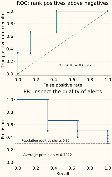
Two curves for the same ten ranked cases. ROC AUC is 0.8095. The precision–recall curve has average precision 0.7222, with a horizontal reference at positive prevalence 0.30. — Both plots use the same scores and labels. The ROC diagonal ($0.50$) represents class-independent random ranking; the PR horizontal baseline equals the population positive prevalence $\pi$.

ROC AUC is the probability $\Pr(\hat s_+ > \hat s_-)$ that a randomly selected positive outranks a randomly selected negative (counting ties as $\frac12$; here $17 / 21 \approx 0.8095$). Average precision (AP / PR-AUC) summarizes precision at each newly recovered positive: here $(1/1 + 2/3 + 3/6) / 3 \approx 0.7222$.

AP is not every quantity called “PR AUC”

Let $R_n$ and $P_n$ be recall and precision after admitting the next score group, starting from $R_0=0$. Each recall gain weights the precision at that step:

$$\operatorname{AP}=\sum_n(R_n-R_{n-1})P_n.$$

Scikit-learn’s average_precision_score uses this non-interpolated convention. Applying trapezoidal integration to the PR points gives about 0.6778 for this same example, not 0.7222. Report the function or interpolation convention when naming a PR area.

Neither area selects the operating threshold for you. Compare the region relevant to the task, then choose the decision rule on validation data. The threshold chapter keeps that selection separate from the final test.

Ranking quality does not establish probability quality

A score can rank cases correctly while being overconfident. Calibration asks whether cases assigned, for example, 20% probability are positive about 20% of the time. Examine a reliability diagram and probability-sensitive scores such as log loss or Brier score when probabilities inform downstream decisions.

Under severe imbalance, also show the number of cases and positives behind each calibration bin. A bin containing almost no positives provides weak evidence. A single probability score mixes several properties, so it does not replace the reliability plot. Fit any calibration model using suitable held-out or cross-validated predictions, not the final test labels.

References and further reading

Scikit-learn: classification metrics — confusion-based metrics, averaging conventions and ROC evaluation.
Scikit-learn: average_precision_score — non-interpolated AP and its distinction from trapezoidal integration.
Scikit-learn: precision_recall_curve — threshold groups, output arrays and plotting endpoints.
Scikit-learn: probability calibration — reliability diagrams and the separation between calibration and other probability-score properties.
Imbalanced-learn: resampling pitfalls — evaluation prevalence and the training boundary.