Deep Learning · Data Imbalance in Deep LearningChapter 08 / 12

Cost-Sensitive Cross-Entropy, Effective Number of Samples, and Focal Loss

October 2026 · 7 min read

Derive Cui et al.’s Effective Number of Samples $E_n=(1-\beta^n)/(1-\beta)$ from overlapping feature volume, and derive Focal Loss $-\alpha_t(1-p_t)^\gamma\log p_t$ and its exact logit gradient.

Instead of changing the data loader, loss-reweighting methods keep standard sampling and multiply each example’s loss by a weight. That weight can depend on class rarity (Cost-Sensitive Cross-Entropy and Effective Number of Samples) or on prediction hardness (Focal Loss).

1. Cost-sensitive cross-entropy and why raw $1/n_k$ weights overshoot

Class-weighted cross-entropy assigns a positive scalar weight $\alpha_y>0$ to the true class $y\in\{1,\dots,K\}$:

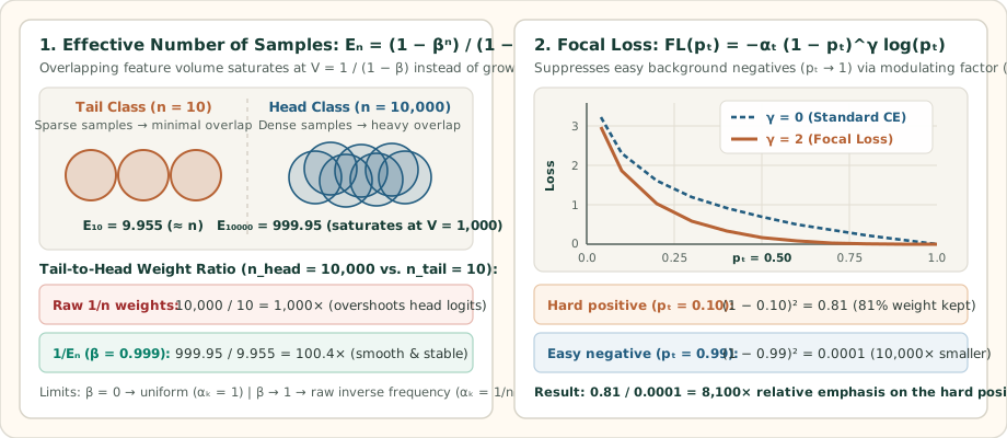
$$L_{\text{WCE}}(z,y)=-\alpha_y\log p_y,\qquad\frac{\partial L_{\text{WCE}}}{\partial z_k}=\alpha_y\bigl(p_k-\mathbf{1}[k=y]\bigr).$$

Notice that multiplying a sample’s loss by $\alpha_y$ multiplies all $K$ coordinates of its logit gradient by $\alpha_y$: a tail example not only pulls its own logit $z_y$ up $\alpha_y$ times harder, it also pushes every competing head logit $z_k$ ($k\ne y$) down $\alpha_y$ times harder. When $\alpha_y=1/n_y$ on a dataset with $n_{\text{head}}=10{,}000$ and $n_{\text{tail}}=10$, a single misclassified tail example receives a $1000\times$ larger gradient step than a head example, causing wild logit oscillations and false positives.

2. Cui et al.’s Effective Number of Samples: $E_n=\frac{1-\beta^n}{1-\beta}$

Why is $10{,}000$ head examples not $1000\times$ more informative than $10$ tail examples? Because nearby training examples overlap! Cui et al. (CVPR 2019) model the feature space of a class as a total volume $V\ge 1$, where each training sample covers a unit volume of $1$ and overlaps a previously covered region with probability $p=E_{n-1}/V$:

$$\begin{aligned}E_n&=\underbrace{E_{n-1}}_{\text{already covered}}+\underbrace{\left(1-\frac{E_{n-1}}{V}\right)\cdot 1}_{\text{newly covered volume}}=1+\left(1-\frac{1}{V}\right)E_{n-1}.\end{aligned}$$

Define $\beta=1-\frac{1}{V}\in[0,1)$ (so $V=\frac{1}{1-\beta}$). Unrolling the recurrence from $E_1=1$ yields a geometric series—the Effective Number of Samples $E_n$:

$$\begin{aligned}E_n&=1+\beta+\beta^2+\cdots+\beta^{n-1}=\frac{1-\beta^n}{1-\beta},\qquad\alpha_k=\frac{1}{E_{n_k}}=\frac{1-\beta}{1-\beta^{n_k}}.\end{aligned}$$

Check the two endpoints and a concrete numerical comparison at $\beta=0.999$ ($V=1000$) for $n_{\text{head}}=10{,}000$ vs. $n_{\text{tail}}=10$:

$$\begin{aligned}\beta=0:&\quad E_n=1\implies\alpha_k=1\quad(\text{uniform unweighted CE}),\\[4pt]\beta\to 1:&\quad \lim_{\beta\to 1}\frac{1-\beta^n}{1-\beta}=n\implies\alpha_k=\frac{1}{n_k}\quad(\text{raw inverse frequency}),\\[6pt]\beta=0.999:&\quad E_{10000}=\frac{1-0.999^{10000}}{1-0.999}\approx 999.95,\qquad E_{10}=\frac{1-0.999^{10}}{1-0.999}\approx 9.955\implies\frac{\alpha_{\text{tail}}}{\alpha_{\text{head}}}\approx 100.4\times\text{ (instead of }1000\times\text{)}.\end{aligned}$$

Left: overlapping volume model for Effective Number of Samples E_n = (1 - beta^n)/(1 - beta). Right: Focal Loss curve showing (1 - p_t)^gamma suppressing easy negatives. — Left: head classes have heavy sample overlap so their effective volume saturates at $1/(1-\beta)$, preventing $1/E_n$ weights from exploding. Right: Focal Loss multiplies cross-entropy by $(1-p_t)^\gamma$, shrinking the loss of well-classified negatives ($p_t=0.99$) by $10{,}000\times$ at $\gamma=2$.

3. Focal Loss: down-weight easy examples via $(1-p_t)^\gamma$

Class weights treat every majority example equally—even when $99\%$ of majority examples are already classified with $p_t=0.99$ and still add up to dominate the gradient. Lin et al. (ICCV 2017) define $p_t$ as the model’s predicted probability for the ground-truth class ($p_t=p$ if $y=1$, and $p_t=1-p$ if $y=0$) and multiply cross-entropy by the modulating factor $(1-p_t)^\gamma$ with focusing parameter $\gamma\ge 0$:

$$\operatorname{FL}(p_t)=-\alpha_t(1-p_t)^\gamma\log(p_t).$$

To derive the exact gradient with respect to the logit $z$, let $y\in\{\pm 1\}$ so $p_t=\sigma(yz)$ and $\frac{\partial p_t}{\partial z}=y\,p_t(1-p_t)$. Applying the product rule to $-(1-p_t)^\gamma\log p_t$ gives:

$$\begin{aligned}\frac{\partial\operatorname{FL}}{\partial z}&=-\alpha_t\frac{\partial}{\partial p_t}\Bigl[(1-p_t)^\gamma\log p_t\Bigr]\frac{\partial p_t}{\partial z}\\[6pt]&=-\alpha_t\left[-\gamma(1-p_t)^{\gamma-1}\log p_t+\frac{(1-p_t)^\gamma}{p_t}\right]y\,p_t(1-p_t)\\[6pt]&=-y\,\alpha_t(1-p_t)^\gamma\Bigl(1-p_t-\gamma\,p_t\log p_t\Bigr).\end{aligned}$$

Worked numerical check ($\gamma=2$ vs. $\gamma=0$): Compare an easy background negative ($p_t=0.99$) against a hard minority positive ($p_t=0.10$):

$$\begin{aligned}\text{Easy negative }(p_t=0.99):&\quad (1-p_t)^2=(0.01)^2=0.0001\quad\bigl(\text{loss reduced by }10{,}000\times\bigr),\\[4pt]\text{Hard positive }(p_t=0.10):&\quad (1-p_t)^2=(0.90)^2=0.8100\quad\bigl(\text{retains }81\%\text{ of full CE weight}\bigr),\\[4pt]\text{Relative importance ratio}:&\quad \frac{0.8100}{0.0001}=8{,}100\times\text{ in favor of the hard positive!}\end{aligned}$$

4. Questions worth answering

Why can high $\gamma$ ($\gamma\ge 3$) hurt training when the dataset contains mislabeled examples (label noise)?

A mislabeled example has a tiny predicted probability $p_t\ll 1$ for its corrupted label, so $(1-p_t)^\gamma\approx 1$ keeps its weight near maximum while clean examples are down-weighted by $(1-p_t)^\gamma\ll 1$. As a result, Focal Loss concentrates the gradient on corrupted labels.

In Class-Balanced Loss, how should you choose $\beta$?

Since $V=\frac{1}{1-\beta}$ represents the effective feature-space capacity per class, $\beta\in\{0.99, 0.999, 0.9999\}$ corresponds to saturating at $V\in\{100, 1000, 10000\}$ unique prototypes per class.