1. Vision Transformer (ViT) from First Principles: Patchify, Stride-$P$ Conv2d Projection, [CLS] Token, 2D Positional Interpolation & Inductive Biases
Before 2020, computer vision was synonymous with Convolutional Neural Networks (CNNs) because 2D convolutions bake in two powerful spatial priors—local connectivity and translation equivariance—while keeping compute linear in pixel count. When Dosovitskiy et al. (2020) introduced the Vision Transformer (ViT) in An Image is Worth 16x16 Words, their core design principle was radical minimalism: change as little of Vaswani et al.'s (2017) standard NLP Transformer Encoder as possible. By partitioning an image of size $H \times W \times C$ into $N = (H/P)(W/P)$ non-overlapping patches of $P \times P$ pixels and linearly projecting each patch into a $d$-dimensional vector, an image becomes a short 1D sequence of $N$ visual "words."
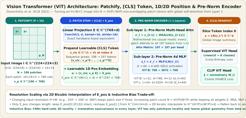
[CLS] tokens and $L$ Pre-Norm Transformer Encoder layers.1. Why Patches Instead of Pixels? The Quadratic Bottleneck
In standard scaled dot-product self-attention over a sequence of $n$ tokens, every token queries every other token, forming an $n \times n$ attention matrix per head per layer. If we treat each pixel of an RGB image $\mathbf{I} \in \mathbb{R}^{H \times W \times C}$ as an individual token, then for a modest $224 \times 224$ image:
Even in `float16` ($2\text{ bytes}$ per element), storing a single layer's attention scores across $H = 12$ heads for batch size $B = 1$ would require $12 \times 2.52 \times 10^9 \times 2 \approx 60.4\text{ GB}$ of VRAM—before accounting for gradients or activations.
By grouping pixels into non-overlapping square patches of side length $P$, ViT reduces the sequence length by a factor of $P^2$ and reduces the quadratic attention matrix size by a factor of $P^4$:
For $H = W = 224$ and $P = 16$, $P^2 = 256$ and $P^4 = 65{,}536$:
- Grid dimensions: $(224 / 16) \times (224 / 16) = 14 \times 14 = 196$ patches.
- Attention matrix per head (including the prepended
[CLS]token): $197 \times 197 = 38{,}809$ entries—a $64{,}872\times$ reduction in attention memory and FLOPs compared to pixel-level attention!
2. Patchify Math & Exact Equivalence to Stride-$P$ Conv2d
Let the input image be $\mathbf{I} \in \mathbb{R}^{H \times W \times C}$ where $H$ and $W$ are divisible by the patch size $P$. We partition $\mathbf{I}$ into $N = (H/P)(W/P)$ non-overlapping spatial blocks and flatten each $P \times P \times C$ block into a row vector $\mathbf{x}_p^{(i)} \in \mathbb{R}^{P^2 C}$ for $i \in \{1, \dots, N\}$:
For ViT-Base/16 (`ViT-B/16`) on a $224 \times 224 \times 3$ image:
- Each flattened patch has dimension $P^2 C = 16 \times 16 \times 3 = 768$.
- A learnable linear projection matrix $E \in \mathbb{R}^{(P^2 C) \times d}$ (plus optional bias $\mathbf{b} \in \mathbb{R}^d$) maps each flattened patch into the Transformer's hidden width $d$: $$\mathbf{e}_i = \mathbf{x}_p^{(i)} E + \mathbf{b} \in \mathbb{R}^d, \qquad i = 1, \dots, N$$
Why Every Production Codebase Uses nn.Conv2d(C, d, kernel_size=P, stride=P)
Explicitly slicing an image tensor into patches via `einops.rearrange` or `unfold` and multiplying by $E \in \mathbb{R}^{(P^2 C) \times d}$ requires materializing an intermediate patch buffer in memory. However, consider what a 2D convolution with kernel size $P \times P$ and stride $P$ computes at spatial grid coordinates $(r, c) \in \{0, \dots, H/P - 1\} \times \{0, \dots, W/P - 1\}$ for output channel $k \in \{1, \dots, d\}$:
Because the stride $P$ equals the kernel width $P$, the convolutional receptive fields are strictly non-overlapping and tile the image identically to the patch grid! Reshaping the 4D convolutional output $[B, d, H/P, W/P] \to [B, d, N] \to [B, N, d]$ yields the exact same tensor as flattening patches and applying `nn.Linear(P*P*C, d)`, while leveraging highly optimized cuDNN implicit-GEMM kernels without allocating an intermediate `unfold` buffer.
Worked Numerical Example (Toy $4 \times 4$ Single-Channel Image, $P = 2$, $d = 3$)
Suppose $H = W = 4$, $C = 1$, and patch size $P = 2$, giving $N = (4/2)(4/2) = 4$ patches, each of flattened length $P^2 C = 4$:
With projection matrix $E \in \mathbb{R}^{4 \times 3}$ and zero bias:
3. The Learnable [CLS] Token & 1D/2D Positional Embeddings
Following BERT (Devlin et al., 2019), Dosovitskiy et al. prepend a learnable class token $\mathbf{x}_{\text{cls}} \in \mathbb{R}^{1 \times d}$ to the sequence of $N$ projected patch embeddings. Why prepend a dedicated synthetic token instead of just picking one of the $N$ patch tokens at the output?
- Spatial neutrality: Every patch token $\mathbf{e}_i$ is initialized with the pixels of a specific $P \times P$ region $(r, c)$. Using patch $i$ as the global image representation would bias the classifier toward that corner or center region.
- Dedicated global scratchpad: Because $\mathbf{x}_{\text{cls}}$ is tied to no spatial patch, its queries $\mathbf{q}_{\text{cls}}^{(\ell)}$ in every layer $\ell = 1, \dots, L$ are free to aggregate task-relevant visual evidence across all $N$ patches unbiased by local pixel input.
After prepending $\mathbf{x}_{\text{cls}}$, the sequence has length $N + 1$. Because self-attention is permutation-equivariant—permuting the $N$ patches in the input simply permutes the output rows without changing any attention weights—spatial geometry must be injected explicitly via a learnable positional embedding table $\mathbf{E}_{\text{pos}} \in \mathbb{R}^{(N+1) \times d}$:
Why Does 1D Learnable Position Embedding Match 2D-Aware Embeddings in ViT?
Dosovitskiy et al. (Appendix D.4) ablated four positional encoding strategies on ImageNet:
- No positional embedding: Treating the image as an unordered "bag of $16 \times 16$ patches." Accuracy drops by more than $3\%$, proving spatial arrangement matters beyond patch-internal structure.
- 1D learnable positional embedding ($\mathbf{E}_{\text{pos}} \in \mathbb{R}^{(N+1) \times d}$): Raster-scan indexing $0, 1, \dots, N$.
- 2D-aware learnable positional embedding: Separate learnable row embeddings $\mathbf{E}_{\text{row}} \in \mathbb{R}^{(H/P) \times (d/2)}$ and column embeddings $\mathbf{E}_{\text{col}} \in \mathbb{R}^{(W/P) \times (d/2)}$ concatenated into $\mathbb{R}^d$ at each grid cell $(r, c)$.
- Relative 2D positional bias: Encoding pairwise grid distances $(\Delta r, \Delta c)$ directly inside attention logits.
Surprisingly, 1D learnable, 2D-aware, and relative 2D embeddings all achieved virtually identical accuracy (within $0.2\%$). Why? At $14 \times 14 = 196$ patches, there are only $14$ rows and $14$ columns—so learning the 2D grid topology from scratch requires discovering that index $i + 1$ is the horizontal neighbor and index $i + 14$ is the vertical neighbor. Visualizing the cosine similarity matrix $\mathbf{E}_{\text{pos}}[1:] \mathbf{E}_{\text{pos}}[1:]^\top \in \mathbb{R}^{196 \times 196}$ of a trained 1D ViT reveals unmistakable 2D periodic stripes: each patch's learned 1D position vector has highest cosine similarity with patches in the same row and the same column!
4. The $L$-Layer Pre-Norm Transformer Encoder Stack
Unlike Vaswani et al. (2017), which placed LayerNorm after the residual addition (Post-Norm), ViT uses the Pre-Norm formulation (Wang et al., 2019; Radford et al., 2019) where LayerNorm is applied to the input of each sub-layer while the identity residual highway remains completely unobstructed from $\mathbf{z}_0$ to $\mathbf{z}_L$:
Inside each Multi-Head Self-Attention ($\operatorname{MSA}$) block with $H$ heads of dimension $d_h = d / H$, let $\tilde{\mathbf{z}} = \operatorname{LN}(\mathbf{z}_{\ell-1}) \in \mathbb{R}^{(N+1) \times d}$:
Crucially, unlike autoregressive language models (GPT), ViT applies bidirectional (unmasked) self-attention: every patch token can attend to every other patch token (top-left corner to bottom-right corner) starting in Layer 1.
5. Patch Size Scaling ($P = 32, 16, 14$) & 2D Bicubic Positional Interpolation
Notice that the parameter count of the Transformer Encoder ($L$ blocks of $\operatorname{MSA}$ and $\operatorname{MLP}$) depends only on the hidden dimension $d$ and layer count $L$, not on the patch size $P$ or image resolution $H \times W$. Shrinking $P$ slightly decreases the patch stem parameters ($P^2 C d$), yet explodes the compute FLOPs because token length $N = (H/P)(W/P)$ grows quadratically as $P$ shrinks:
| Configuration | Input Resolution | Patch Grid $(H/P) \times (W/P)$ | Sequence Length $N+1$ | Attention Pairs $(N+1)^2$ | Relative Compute |
|---|---|---|---|---|---|
| ViT-B/32 | $224 \times 224$ | $7 \times 7 = 49$ | $50$ | $2{,}500$ | $1.0\times$ (fastest) |
| ViT-B/16 | $224 \times 224$ | $14 \times 14 = 196$ | $197$ | $38{,}809$ | $\sim 4.4\times$ |
| ViT-B/14 | $224 \times 224$ | $16 \times 16 = 256$ | $257$ | $66{,}049$ | $\sim 6.1\times$ |
| ViT-B/16 @ $384\text{px}$ | $384 \times 384$ | $24 \times 24 = 576$ | $577$ | $332{,}929$ | $\sim 16.5\times$ |
Fine-Tuning at Higher Resolution via 2D Bicubic Interpolation of $\mathbf{E}_{\text{pos}}$
In practice, pretraining happens at $224 \times 224$ for throughput, followed by fine-tuning at a higher resolution $H' \times W'$ (such as $384 \times 384$ in supervised ViT, or $336 \times 336$ in CLIP ViT-L/14@336px). When we keep patch size $P$ fixed and increase image resolution from $(H, W)$ to $(H', W')$:
- The patch projection `Conv2d(3, d, kernel_size=P, stride=P)` and all $L$ Transformer blocks operate on per-token dimension $d$, so their weights require zero shape changes.
- The patch count increases from $N = (H/P)(W/P)$ to $N' = (H'/P)(W'/P)$ (e.g., for $P=16$ from $224^2 \to 384^2$, the grid grows from $14 \times 14 = 196$ to $24 \times 24 = 576$ patches).
- The pretrained positional embedding $\mathbf{E}_{\text{pos}} \in \mathbb{R}^{(N+1) \times d}$ only has $197$ rows, whereas we now need $577$ rows. To preserve the learned 2D geometry:
- Separate the
[CLS]position vector $\mathbf{e}_{\text{pos}}^{\text{cls}} = \mathbf{E}_{\text{pos}}[0:1, :] \in \mathbb{R}^{1 \times d}$. - Reshape the remaining $N$ patch position vectors $\mathbf{E}_{\text{pos}}[1:, :] \in \mathbb{R}^{N \times d}$ back into a 2D spatial grid of shape $\left[\frac{H}{P}, \frac{W}{P}, d\right]$ (e.g., $14 \times 14 \times 768$).
- Apply 2D bicubic interpolation along the two spatial axes to resize $\left[\frac{H}{P}, \frac{W}{P}, d\right] \to \left[\frac{H'}{P}, \frac{W'}{P}, d\right]$ (e.g., $24 \times 24 \times 768$).
- Flatten back to $\mathbb{R}^{N' \times d}$ and concatenate $\mathbf{e}_{\text{pos}}^{\text{cls}}$ at index $0$ to obtain $\tilde{\mathbf{E}}_{\text{pos}} \in \mathbb{R}^{(N'+1) \times d}$.
- Separate the
6. Inductive Biases: Why CNNs Win on Small Data and ViT Wins at Scale
Why did Dosovitskiy et al. find that ViT slightly underperformed ResNets (BiT) when trained from scratch on mid-sized ImageNet-1k ($1.28\text{M}$ images), matched ResNets on ImageNet-21k ($14\text{M}$ images), and decisively surpassed ResNets when pretrained on JFT-300M ($300\text{M}$ images) or WIT-400M (CLIP)?
- CNN Inductive Biases (Hard-Coded Geometry): Every $3 \times 3$ convolution enforces locality (a neuron only sees a $3 \times 3$ neighborhood) and translation equivariance (the exact same filter weights are shared across all $(x, y)$ coordinates). A CNN cannot help but learn local edge and texture detectors first, building global receptive fields only gradually with depth. This restricts the hypothesis space, preventing overfitting on small datasets ($1\text{M}$ images).
- ViT Inductive Biases (Minimalist Geometry): In ViT, only the initial patch split ($P \times P$), the MLP (applied independently per patch), and the 2D bicubic interpolation of $\mathbf{E}_{\text{pos}}$ carry 2D spatial structure. The self-attention layers are completely global and position-agnostic from Layer 1.
- Mean Attention Distance (Dosovitskiy et al., Figure 7): By measuring the attention-weighted pixel distance $\sum_j A_{ij} \|\mathbf{p}_i - \mathbf{p}_j\|_2$ for each head across depth, Dosovitskiy et al. discovered that in a well-trained ViT, early layers split their heads: some heads attend strictly locally (small mean distance, acting like learned $3 \times 3$ or $5 \times 5$ convolutions), while other heads in Layer 1 already attend across the entire $224 \times 224$ image ($>100\text{px}$ mean distance)! By Layer 10–12, almost all heads integrate global context.
7. Clean PyTorch Implementation of Standard ViT + 2D Pos Interpolation
import torch
import torch.nn as nn
import torch.nn.functional as F

class VisionTransformer(nn.Module):
    """
    Standard Vision Transformer (Dosovitskiy et al., ICLR 2021)
    with dynamic 2D bicubic positional embedding interpolation.
    """
    def __init__(
        self,
        img_size: int = 224,
        patch_size: int = 16,
        in_chans: int = 3,
        num_classes: int = 1000,
        embed_dim: int = 768,
        depth: int = 12,
        num_heads: int = 12,
        mlp_ratio: float = 4.0,
        drop_rate: float = 0.1,
    ):
        super().__init__()
        self.img_size = img_size
        self.patch_size = patch_size
        self.grid_size = img_size // patch_size
        self.num_patches = self.grid_size * self.grid_size

        # 1. Patchify + Linear Projection fused as a stride-P Conv2d
        self.patch_embed = nn.Conv2d(
            in_chans, embed_dim, kernel_size=patch_size, stride=patch_size, bias=True
        )

        # 2. Learnable [CLS] token and 1D Positional Embeddings
        self.cls_token = nn.Parameter(torch.zeros(1, 1, embed_dim))
        self.pos_embed = nn.Parameter(torch.zeros(1, self.num_patches + 1, embed_dim))
        self.pos_drop = nn.Dropout(p=drop_rate)

        # 3. L Pre-Norm Transformer Encoder Blocks
        encoder_layer = nn.TransformerEncoderLayer(
            d_model=embed_dim,
            nhead=num_heads,
            dim_feedforward=int(embed_dim * mlp_ratio),
            dropout=drop_rate,
            activation="gelu",
            batch_first=True,
            norm_first=True,  # Pre-Norm: LN before MSA and MLP
        )
        self.blocks = nn.TransformerEncoder(encoder_layer, num_layers=depth)

        # 4. Final LayerNorm on [CLS] and Classification Head
        self.norm = nn.LayerNorm(embed_dim, eps=1e-6)
        self.head = nn.Linear(embed_dim, num_classes)

        nn.init.trunc_normal_(self.pos_embed, std=0.02)
        nn.init.trunc_normal_(self.cls_token, std=0.02)

    def interpolate_pos_encoding(self, x: torch.Tensor, H: int, W: int) -> torch.Tensor:
        """2D bicubic interpolation of patch position embeddings when H, W != img_size."""
        N = x.shape[1] - 1
        if N == self.num_patches and H == W:
            return self.pos_embed

        cls_pos = self.pos_embed[:, :1]       # [1, 1, d]
        patch_pos = self.pos_embed[:, 1:]     # [1, N_orig, d]
        d = x.shape[-1]
        h_new, w_new = H // self.patch_size, W // self.patch_size

        # Reshape [1, g, g, d] -> permute [1, d, g, g] -> bicubic resize -> [1, h_new*w_new, d]
        patch_pos = patch_pos.reshape(1, self.grid_size, self.grid_size, d).permute(0, 3, 1, 2)
        patch_pos = F.interpolate(
            patch_pos, size=(h_new, w_new), mode="bicubic", align_corners=False
        )
        patch_pos = patch_pos.permute(0, 2, 3, 1).flatten(1, 2)
        return torch.cat((cls_pos, patch_pos), dim=1)

    def forward(self, x: torch.Tensor) -> torch.Tensor:
        B, C, H, W = x.shape
        # [B, 3, H, W] -> [B, d, H/P, W/P] -> [B, d, N] -> [B, N, d]
        x = self.patch_embed(x).flatten(2).transpose(1, 2)

        # Prepend [CLS] token: [B, 1, d] + [B, N, d] -> [B, N+1, d]
        cls_tokens = self.cls_token.expand(B, -1, -1)
        x = torch.cat((cls_tokens, x), dim=1)

        # Add (interpolated) positional embeddings
        x = self.pos_drop(x + self.interpolate_pos_encoding(x, H, W))

        # L Pre-Norm Transformer blocks
        x = self.blocks(x)

        # Readout from [CLS] at index 0
        cls_out = self.norm(x[:, 0])
        return self.head(cls_out)